
Abstract
Globally, economic losses from flooding exceeded $19 billion in 2012, and are rising rapidly. Hence, there is an increasing need for global-scale flood risk assessments, also within the context of integrated global assessments. We have developed and validated a model cascade for producing global flood risk maps, based on numerous flood return-periods. Validation results indicate that the model simulates interannual fluctuations in flood impacts well. The cascade involves: hydrological and hydraulic modelling; extreme value statistics; inundation modelling; flood impact modelling; and estimating annual expected impacts. The initial results estimate global impacts for several indicators, for example annual expected exposed population (169 million); and annual expected exposed GDP ($1383 billion). These results are relatively insensitive to the extreme value distribution employed to estimate low frequency flood volumes. However, they are extremely sensitive to the assumed flood protection standard; developing a database of such standards should be a research priority. Also, results are sensitive to the use of two different climate forcing datasets. The impact model can easily accommodate new, user-defined, impact indicators. We envisage several applications, for example: identifying risk hotspots; calculating macro-scale risk for the insurance industry and large companies; and assessing potential benefits (and costs) of adaptation measures.
Export citation and abstract BibTeX RIS

Content from this work may be used under the terms of the Creative Commons Attribution 3.0 licence. Any further distribution of this work must maintain attribution to the author(s) and the title of the work, journal citation and DOI.
1. Introduction
Globally, economic losses from flooding exceeded $19 billion in 2012 (Munich Re 2013), and have risen over the past half century (IPCC 2012, UNISDR 2011, Visser et al 2012). Hence, recent years have seen increased attention for strategic flood risk assessments6, and their inclusion in global integrated assessments (e.g. OECD 2012). For example, in 2005 the World Bank Hotspots project estimated risk based on reported flood event data combined with gridded population and GDP (Dilley et al 2005). UNISDR produced maps of population and GDP exposed to flooding using a combination of modelled and reported events (Peduzzi et al 2009, UNISDR 2009). Jongman et al (2012a) contributed further by quantifying changes in population and assets exposed to 100-year flood events between 1970 and 2050.
Due to the high computational costs of producing flood hazard maps generally (Gouldby and Kingston 2007, Apel et al 2008), let alone globally, past studies have assessed risk based on very limited numbers of hazard maps. This brings several problems. Firstly, many stakeholders require risk-based information in terms of annual expected impacts (e.g. annual expected damage or mortality). For this, impacts must be calculated for several return-periods, and annual expected impacts estimated as the integral of the area under an exceedance probability–impact curve (Meyer et al 2009). These estimates are highly sensitive to the return-periods used (Ward et al 2011). Secondly, the limited number of hazard maps means that past global risk studies have not assessed sensitivity of results to the input data.
Pappenberger et al (2012) developed a model cascade to produce hazard maps for several return-periods (2–500 years), showing flooded fraction for 25 km × 25 km grid-cells. However, they were not used to estimate risk. Winsemius et al (2013) developed a framework for global flood risk assessment, leading to a method for producing hazard maps at 30'' × 30'' resolution (about 1 km × 1 km at the equator). The method was consequently demonstrated for Bangladesh, for floods with return-periods up to 30 years. However, extrapolation to more extreme events was not attempted, and no global assessment was carried out. Hirabayashi et al (2013) quantified the impacts of future climate change on the number of people exposed to 10 and 100-year flood events, but did not calculate annual expect impacts or impact indicators other than population.
To address these issues, we have improved and extended the model cascade of Winsemius et al (2013), so that it now produces global-scale flood risk maps based on a large number of return-periods. We have also developed a module to simulate multiple risk indicators (other than economic damage), which can easily accommodate new indicators required by end-users. In this letter we: (a) describe the model cascade; (b) present global risk results; and (c) assess the sensitivity of the results to several input parameters (climate input data, extreme value distributions, and flood protection standards).
2. Setup of model cascade
Our method involves a cascade of models or steps, which are described in this section. For those models or steps described in Winsemius et al (2013) or elsewhere, only a brief overview is given. An overview is shown in figure 1.

Figure 1. Flowchart showing the main flow of data and models used in this study.
Download figure:
Standard image High-resolution image2.1. Global hydrological and hydraulic modelling
We simulated daily discharges and flood volumes (0.5° × 0.5°) using the global hydrological model PCR-GLOBWB (Van Beek and Bierkens 2009, Van Beek et al 2011), and its extension for dynamic routing, DynRout (PCR-GLOBWB-DynRout). Discharge arises from flood-wave propagation; in each cell the associated flood volume is stored in the channel or on the floodplain in case of overbank flooding. The suitability of these models is discussed in Winsemius et al (2013). In brief, the model runs on a daily time-step, which is sufficiently short for runoff generation and flood propagation. It is also capable of using a radiation-based potential evapotranspiration scheme. Two other important features are that the runoff scheme resolves infiltration excess as a non-linear function of soil moisture; and the routing differentiates river flow from overbank flow dynamically.
The models were forced by meteorological fields (precipitation, temperature, radiation) for 1958–2000 from the EU-WATCH project (Weedon et al 2011). The WATCH forcing data (WFD) were derived from the ERA-40 reanalysis product (Uppala et al 2006) via sequential interpolation to a horizontal resolution of 0.5° × 0.5°, with elevation corrections and monthly-scale adjustments of daily values to reflect CRU (temperature and cloud-cover) and GPCC (precipitation) monthly observations. They were also combined with new corrections for varying atmospheric aerosol-loading and separate precipitation gauge corrections. Specifically, we used the following datasets: air temperature, rainfall and snow (monthly bias-corrected by GPCC rainfall), and the Penman–Monteith based potential evaporation estimates. We aggregated all fields to daily values. Although WFD are available for 1901–2000, the pre-1958 dataset was developed by reordering the data for the later 1958–2000 period, prior to bias correction. Hence, we chose to use the later period, which represents actual years.
2.2. Extreme value statistics
In Winsemius et al (2013), a 30-year time-series of daily flood volumes was used to derive the maximum flood volume per grid-cell, which was assumed to represent a 30-year return-period. In the current paper, we developed inundation maps for different return-periods based on the Gumbel distribution. From the daily flood volume time-series, we extracted an annual time-series of maximum flood volumes for hydrological years 1958–2000.7 For each cell, we then fit a Gumbel distribution through this time-series, based on non-zero data (extracting Gumbel parameters for the best-fit and the 5 and 95% confidence limits). For cells in which zero flood volume was simulated in one or more years, we also calculated the exceedance probability of zero flood volume. These Gumbel parameters were used to calculate flood volumes per grid-cell for selected return-periods (2, 5, 10, 25, 50, 100, 250, and 1000 years). Flood volumes were calculated conditional to the exceedance probability of zero flood volume. For those cells where fewer than five non-zero data points were available, flood volume was assumed to be zero.
2.3. Inundation modelling
The following step is the conversion of the coarse resolution flood volumes into high resolution (30'' × 30'') hazard maps showing inundation depths.
This is carried out using the GLOFRIS downscaling module described in Winsemius et al (2013). In brief, the module includes a high resolution digital elevation model (30'' × 30'') and a map of river cells at the same resolution. For each 0.5° × 0.5° grid-cell, the module iteratively imposes water levels, in steps of 10 cm, above the elevation of each river-cell in the 30'' × 30'' grid. It then evaluates which upstream connected cells on the high resolution grid have an elevation lower than the imposed water level in the river channel. These cells receive a layer of flood water, equal to the water level minus the elevation of the cell being considered. This process is iterated (with steps of 10 cm) until the flood volume generated for the cell in the low resolution model (0.5° × 0.5°) has been depleted.
We assumed that flood volumes with 2-year return-period would not lead to overbank flooding (Dunne and Leopold (1978) estimate bankfull discharge to have an average return-period of about 1.5 years). Hence, this flood volume is first subtracted from the flood volumes for the different return-periods (5, 10, 25 year, etc), before the inundation downscaling is carried out. In practice, this means that any systematic overestimation of 2-year flood volume (whether that be related to the input climate data, hydrological–hydraulic modelling, or the use of extreme value statistics) is subtracted from the flood volumes for all return-periods.
2.4. Impact modelling
We have developed a flood impact module that estimates impacts per 30'' × 30'' grid-cell for different return-periods, and aggregates to any user-defined geographical unit (e.g. countries, basins). The module has been developed to accommodate new impact indicators required by end-users. To date, the following indicators have been integrated: affected population, affected GDP, affected agricultural value, economic urban asset exposure, and urban damage (see following paragraphs).
2.4.1. Affected population and affected GDP.
Affected population and GDP are estimated using downscaled population and GDP data for 2010 (Van Vuuren et al 2007). The maps are produced at 0.5° × 0.5°, based on population scenarios for 26 world regions from the Integrated Model to Assess the Global Environment (IMAGE, Bouwman et al 2006), and 2000 population maps from LandScan 2010 (Bright et al 2010). For GDP, the method assumes convergence of country-level per capita income within a region, evenly distributed over the population within a country. These results are further downscaled to 30'' × 30'' using LandScan (2008)8 population maps. For this letter, we show counts of population and GDP located in inundated cells. However, the affected population module can also give information on the number of people exposed to different (user-defined) inundation depths. This is useful since, for example, an inundation depth of 10 cm clearly has a different impact on human livelihoods than an inundation of 1 m.
2.4.2. Economic urban asset exposure.
This indicator estimates the economic value of exposed assets in urban areas, based on a land use map and a map of estimated urban asset values per square kilometre. The land use data are taken from the HYDE database (Klein Goldewijk et al 2011), which shows the fraction of each grid-cell with urban land cover (5' × 5'). From this, we calculated urban area per cell. We then assigned an economic value to urban area per square kilometre, using Jongman et al (2012a), which is based on GDP-normalised estimates from the Damagescanner model (Klijn et al 2007, Ward et al 2011).
2.4.3. Urban damage.
To demonstrate the influence of using stage-damage functions (representing vulnerability) to estimate urban damages (compared to economic urban asset exposure), we developed a module capable of applying these functions per region. Stage-damage functions show the percentage of exposed assets that would suffer damage for different flood depths (e.g. Merz et al 2010). In this demonstration, we simply apply a stage-damage function representing the average of the high and low urban density land class functions in Damagescanner (the data can be found in supplementary information 1 available at stacks.iop.org/ERL/8/044019/mmedia). This is to demonstrate how the results change compared to those not including a stage-damage function. Clearly, spatial variations in vulnerability can be substantial (Jongman et al 2012b) and future model developments need to incorporate spatially variable functions.
2.4.4. Affected agricultural value.
The value of affected agriculture is calculated using an adapted version of Dilley et al (2005). A map is prepared representing economic agricultural value per grid-cell, and the affected value is calculated as the sum for all flooded cells. Agricultural value per cell is calculated as follows: (a) total value of agriculture per country (as percentage of GDP) is taken from the World Development Indicators of the World Bank9; (b) GDP per country is taken from GISMO (PBL 2008), and combined with (a) to calculate agricultural value per country; (c) agricultural area per cell is calculated using crop density data from HYDE; (d) agricultural value per square kilometre is calculated per country as the total agricultural value of that country divided by agricultural area; and (e) agricultural value per cell is calculated as the value per square kilometre multiplied by agricultural area per cell.
2.5. Estimation of annual expected impacts
Each impact indicator was calculated for the following return-periods: 2, 5, 10, 25, 50, 100, 250, 500, 1000 years, whereby the impact for a 2-year event is always zero. Annual expected impacts were then calculated as the area under the exceedance probability–impact curve (risk curve) (Meyer et al 2009).
3. Results and discussion
3.1. Validation
PCR-GLOBWB has been validated in past studies on discharge (Van Beek et al 2011) and GRACE satellite data of terrestrial water storage (Wada et al 2012). Generally, the model shows fair to good performance. Here, we performed further validation for extreme discharges, since these are strongly related to the flooding process. We used observed daily discharge data from the Global Runoff Data Centre10, using gauging stations with daily data availability for more than 25 years (during 1958–2000), and an upstream area exceeding 125 000 km2. For these stations, and their corresponding cells in PCR-GLOBWB, we estimated discharge for different return-periods. In figure 2, we show the relative error (%) between discharge with a return-period of 10 years (Q10) based on observed and modelled datasets, whereby Q10 is first adjusted for the absolute difference between Q10 and Q2 (similar to the adjustment made in flood volumes)11. Generally, the relative error is reasonable (between −25 and +25% for 37 of the 53 stations). However, large differences can be seen regionally. For example, in several arid regions Q10 is higher in the modelled data. Here, floods are known to re-infiltrate or evaporate from large wetlands such as the inner Niger Delta (Liersch et al 2012) and the Barotse floodplains and Kafue wetlands in the Zambezi (Winsemius et al 2006). Another example is regions where large amounts of water are extracted through reservoir control (e.g. Murray–Darling; see supplementary information 2, available at stacks.iop.org/ERL/8/044019/mmedia). To date, these processes have not been accounted for in our model cascade. In supplementary information 2 we show the Gumbel plots for the modelled and observed data at eight gauging stations covering a range of environmental conditions, and provide a more detailed discussion of the discharge validation results for those stations.
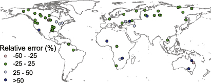
Figure 2. Relative error (%) between discharge with a return-period of 10 years (Q10) derived from modelled and observed data, whereby Q10 is adjusted for the absolute difference between modelled and observed Q2. A positive error indicates an overestimation of the discharge by the model; a negative error indicates an underestimation of the discharge by the model. Results shown for gauging stations with daily data availability for all days on more than 25 years, and with upstream area greater than 125 000 km2.
Download figure:
Standard image High-resolution imageWe also compared our global impact results with reported fatalities and losses from Munich Re's NatCatSERVICE database (Munich Re 2013). To do this, we created inundation maps for each calendar year 1990–2000, and used these to model affected population and exposed urban assets per year. Results are shown in figure 3(a) (exposed population against recorded fatalities) and figure 3(b) (exposed urban assets against reported losses). There is a large absolute difference between these two sets of variables since, as we would expect, the majority of people affected by a flood do not suffer fatality, and not all exposed assets suffer losses. However, we demonstrate here the strong correlation between the variables over the years shown. For exposed population against fatalities, Pearson's r is 0.59, and for exposed urban assets against losses, r is 0.66 (based on de-trended data). This shows that the model cascade captures relative changes in impacts between years well.

Figure 3. Reported and modelled impacts for the periods 1990–2000, whereby reported impacts are taken from the NatCatSERVICE database of Munich Re. Figure 3(a) shows reported fatalities against modelled affected population, and figure 3(b) shows reported losses against modelled urban assets. Pearson's correlation coefficients on the de-trended time-series are 0.59 and 0.66 for (a) and (b) respectively.
Download figure:
Standard image High-resolution imageReported data on global annual expected losses are not available. However, for Europe, the Association of British Insurers estimates current annual average losses from 'extreme flood events' in Europe to be $9–11.5 billion p.a.12 (ABI 2005). Barredo (2009) examined direct economic flood losses in Europe recorded in the EM-DAT database of the Centre of Research on Epidemiology of Disasters (CRED) and Munich Re's NATHAN database, and found annual average losses of $4.1 billion p.a. A direct comparison of these estimates with our own is not straightforward for several reasons. Firstly, it is not clear exactly what loss categories are being referred to in the ABI report. Secondly, there is no definition of what are classed as 'extreme' flood events. Similarly, not all flood events are recorded in the databases. However, we here present a broad comparison with our results, which should be interpreted as an assessment of whether the modelled and reported data show damages in the same order of magnitude. If we assume a 100-year flood protection standard, which is common in Europe according to Wesselink et al (2012), our model suggests annual damages of $9.6 billion. This is within the range estimated by ABI, but higher than that of Barredo (2009). Given the large uncertainties described above, the order of magnitude of the different datasets is similar.
We also compared our simulated annual expected damages in England and Wales with estimates of Hall et al (2005), who used a more detailed country-specific assessment method. Hall et al (2005) simulated average annual damages between about $1 and 3.6 billion p.a. According to Hall et al (2006), roughly half of this relates to river flooding, i.e. $0.5–1.8 billion p.a. Floodplains in England and Wales are not protected against floods with a uniform return-period. In the Thames basin, for example, engineering schemes protect many urban areas against river floods with a return-period of 20–50 years, whilst in some areas there is little to no protection, and in some areas (e.g. London) it is significantly higher (Environment Agency 2009). This makes a direct comparison with our results difficult. However, assuming flood protection standards of 100 years and 10 years, our model simulates annual expected urban damages of ca $0.4 billion p.a. and $2.5 billion p.a. respectively, i.e. of the same order of magnitude as Hall et al (2005).
3.2. Global impact results
Initial results in terms of annual expected impacts are shown in table 1; note that these results assume no flood protection standards (e.g. dikes). In reality many regions are protected by infrastructural measures up to a certain design standard. Clearly, this will lead to an overestimation of impacts. In section 3.4, we provide the first assessment of the sensitivity to the assumption on flood protection standards. From hereon in, all values are shown in USD at purchasing power parity (PPP) in 2010 values.
Table 1. Initial annual expected impact results, assuming no flood protection measures. The results are shown in absolute terms, and relative to total global population (for exposed population) or GDP (all other indicators).
| Impact indicator (annual expected) | Absolute | Relative (%) |
|---|---|---|
| Exposed population—(millions) | 169 | 2.5 |
| Exposed GDP (USD PPP billions) | 1383 | 2.2 |
| Affected agricultural value (USD PPP billions) | 75 | 0.1 |
| Urban damage (USD PPP billions) | 834 | 1.3 |
| Exposed urban assets (USD PPP billions) | 5263 | 8.2 |
The difference between annual expected urban damage and annual expected exposed urban assets is a factor six. Both indicators use the same input data for hazard and exposure, but the former uses a stage-damage function to represent vulnerability. As already stated, we used one stage-damage function for all countries, which is not a true representation of reality. However, it demonstrates the high sensitivity of the results to this assumption.
In figure 4, we show a sample of results spatially, in this case aggregated to the food producing units (FPUs) of IFPRI (International Food Policy Research Institute) and IWMI (International Water Management Institute) (Cai and Rosegrant 2002, Rosegrant et al 2002). Below, we briefly reflect on a number of spatial patterns. The annual expected impact results for all indicators are provided per country and per FPU in the accompanying shapefile in supplementary information 3 and 4 respectively (available at stacks.iop.org/ERL/8/044019/mmedia).

Figure 4. Initial annual expected impacts results per food producing unit (FPU) for several indicators (affected population, affected GDP, affected agricultural value, and urban damage). The left-hand panel shows the results per FPU as a percentage of the global total per indicator. The middle panel shows the results per FPU relative to the total population (for annual exposed population) or GDP (for other indicators) for that particular FPU. The right-hand panel shows the sensitivity of the results to the extrapolation of flood volumes for different return-periods using the Gumbel distribution; the value shown is the range for the 5–95% confidence bounds expressed as a percentage of the value based on the best-fit.
Download figure:
Standard image High-resolution imageIn the left-hand panel of figure 4, values per FPU are shown as a percentage of the global total. Clear geographical differences can be seen between indicators. For example, whilst potential urban damages are highest in large parts of USA, Europe, the eastern coast of Australia, China, and Japan, a different pattern exists for affected population and affected agricultural value. In the latter two, whilst impacts are also very high in China, the percentage shares in USA and Europe are lower, whilst impacts are more highly concentrated in the Indian Subcontinent, south-eastern Asia, and parts of Africa.
In the middle panel of figure 4, annual expected impacts are shown for each FPU relative to the total population (for annual exposed population) or GDP (for other indicators) for that particular FPU. Whilst there are many regions in which impacts may be low in absolute terms, their impact on the given region may be very large. For example, whilst most FPUs in sub-Saharan Africa show low absolute impacts, there are many FPUs where the impacts are amongst the highest relative to their total population or GDP.
3.3. Sensitivity to extreme value statistics and input climate dataset
We assessed the sensitivity of the results to the extrapolation of flood volumes for different return-periods using the Gumbel distribution. To do this, we forced the inundation model with flood volumes obtained for the 5 and 95% confidence bounds of the Gumbel fit for different return-periods, and used the resulting inundation maps as input to the impacts module. The results are shown in figure 5, where blue lines indicate results based on the 5 and 95% confidence limits as a percentage difference compared to those based on the best-fit; this provides an illustration of the uncertainty in the extreme value statistics. Globally, the sensitivity is relatively small, with a range of ca −2 to +5% around the best-fit for exposed population, exposed GDP, and exposed agricultural value, and −5 to +10% for urban damage. The only impact indicator shown for which the depth component of the hazard map is used is the indicator urban damage. Hence, the results are more sensitive to the extrapolation of flood volumes when inundation depths are considered.
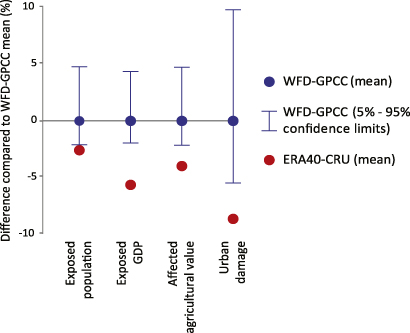
Figure 5. Sensitivity of the initial impact results to the extrapolation of flood volumes for different return-periods using the Gumbel distribution, and to the use of different forcing climate data. The blue lines indicate results based on the 5 and 95% confidence bounds of the Gumbel distribution (based on the EU-WATCH climate input data) as a percentage difference compared to those based on the best-fit. The red circles indicate the results based on the best-fit of the Gumbel distribution based the CRU-ERA40 climate input data.
Download figure:
Standard image High-resolution imageIn figure 4 (right-hand panel), we show this sensitivity per FPU, whereby the value shown per FPU is the range for the 5–95% confidence limits expressed as a percentage of the value based on the best-fit. For most regions the results are relatively insensitive, although again the results for urban damage are higher than for the other indicators. There are several FPUs (for example in North Africa, the Middle East, and around the Kalahari and Gobi deserts) that show a large sensitivity in percentage terms. However, these are FPUs in arid zones in which absolute impacts under the best-fit Gumbel parameters are very small, and where a small increase in absolute terms leads to a large increase in relative terms.
In figure 5, we show an impression of the sensitivity of the global results to the use of a climate forcing dataset that has been subjected to different processing methods. We ran the model cascade for the period 1961–1990 forced firstly with the WATCH forcing data (WFD-GPCC) described previously, and then with ERA-40 data (Uppala et al 2006), bias-corrected based on Sperna Weiland et al (2010). The latter dataset has been bias-corrected using a more simple method, and furthermore, no precipitation undercatch correction has been applied (for details of the procedure see supplementary information 5, available at stacks.iop.org/ERL/8/044019/mmedia). At the global scale, the difference in annual expected impacts between the simulations forced by the CRU-ERA40 data and the WFD-GPCC data is less than 10%. However, an analysis of the differences per FPU shows that the results are highly sensitive at this scale; these results and their discussion can be found in supplementary information 5. Briefly, they show large differences in extreme flood volumes, which appear to be linked to large differences in extreme precipitation between the two datasets. Further research is necessary to examine the influence of a larger range of climate forcing datasets on the impact results, but given the more sophisticated bias correction and the undercatch correction used to create the WFD-GPCC data, these can be assumed to provide the most reliable results.
3.4. Sensitivity to flood protection standards
The results above assume that all flood volumes exceeding a 2-year return-period have the potential to cause flooding, even though many areas are protected by infrastructural measures up to given design standards. Since no global database of protection standards exists, global risk estimates have not been able to incorporate this aspect, meaning that results are likely to be overestimations (in particular those related to high frequency events).
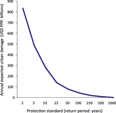
In their study of flood risk in Europe, Feyen et al (2012) accounted for flood protection by truncating the risk curve at a given exceedance probability (corresponding to an assumed protection standard), and estimating annual expected impacts as the integral of the remaining part of the curve. To assess the sensitivity of our results to the use of different protection standards, we also estimated total global impacts using this method. In figure 6, we show how annual expected urban damage decreases as the assumed protection standard increases. Clearly, flood risk estimates are highly sensitive to this parameter. For example, assuming protection standards of 5 and 100 years globally, total simulated annual expected urban damage falls by 41% and 95% respectively. We carried out the same analysis for the other impact indicators, and found very similar results; depending on the indicator, annual expected impacts fall by 48–50% and 95–97% respectively.
Figure 6. Sensitivity of modelled global annual expected urban damage to different assumed flood protection standards.
Download figure:
Standard image High-resolution image
3.5. Main limitations and future work
Our model cascade provides a tool for assessing flood risk in terms of different impact indicators, and its relatively rapid nature allows for the calculation of impacts for many return-periods. However, we have identified several limitations to be addressed in future research. Next to improvements generic to most impact modelling frameworks (e.g. increased spatial resolution of input data, assessing the sensitivity of the results to a larger range of input data sources), we describe several of the main ones below.
Firstly, the hazard maps represent situations with no flood protection measures, whilst we have shown the results to be highly sensitive to such protection standards. Future improvements to the hydrological and hydraulic models will involve the parameterization of measures such as dikes and water retention areas. To date there is no database of such measures available at the global scale. In order to improve the model, we plan to carry out an extensive literature review of protection standards in order to derive spatially disaggregated first order estimates of protection standards at the global scale. Moreover, past research has shown that flood defence fragility (i.e. the reliability of the flood defences conditional on hydraulic loading) can be important in mediating risk (Dawson et al 2005). It would be useful to include simplified estimates of such fragility, using assumptions for broad-scale analyses such as those described in Hall et al (2005).
The modelling approach has been specifically set up to simulate large-scale river floods. To date, it does not include modules for assessing either coastal or pluvial floods, and is not able to capture local-scale flash flood events. In terms of overall risk, all of these floods are of high importance. Indeed, flash flood events often lead to loss of lives, even in areas where fatalities from large-scale river floods are low (e.g. Gaume et al 2009).
The current setup is limited in its treatment of vulnerability. The only impact indicator in the current setup for which vulnerability is explicitly considered is urban damage, and even for this indicator we have used one vulnerability function for all countries. Future model development must concentrate on identifying robust ways of modelling vulnerability at the global scale, for example using stage-damage functions such as those in the CAPRA vulnerability model13, and exploring the use of vulnerability indicators such as those employed by Peduzzi et al (2012), for example considering mortality as a function of total exposed population, and damage as a function of total exposed assets.
To date, we have only examined flood risk under current conditions, and not changes in risk under future scenarios. Generally, uncertainties in absolute flood risk estimates are large (Apel et al 2008, Merz et al 2010, De Moel and Aerts 2011), whilst estimates of relative changes in risk under different scenarios are more robust (e.g. Bubeck et al 2011). Given that our model cascade simulates interannual fluctuations in impacts similar to those in reported loss records, we are confident that it is a useful tool for assessing changes in global risk under future climate and socioeconomic scenarios.
4. Concluding remarks
We have developed and validated a model cascade for producing global-scale flood risk maps, based on large numbers of return-periods. The validation results indicate that it performs adequately, and simulates well the fluctuations in flood impacts between years. Given the relatively small time required to carry out the simulations, and the model cascade's good performance in re-producing flood impact magnitudes between years, it should be well suited for carrying out assessments of relative changes in flood risk in future scenario mode.
An advantage of the model cascade is that it calculates annual expected impacts based on flood hazard simulations for a large number of return-periods. The rapid nature of the cascade also allowed us to provide the first sensitivity assessment of a global flood risk assessment tool. We found the model cascade to be relatively insensitive to the extreme value distribution used to estimate the low frequency flood volumes. However, the results are highly sensitive to the assumed flood protection standard; we highlight the development of a database of such standards at the global scale to be a research priority. Also, the results forced by the more sophisticated WATCH climate forcing data show large differences to those forced by ERA-40 data, which are subjected to a more simple bias correction only.
We envisage several main potential applications of the model. One is the identification of risk hotspots, which is important for planning disaster risk reduction efforts (e.g. UNISDR 2011). Secondly, data on annual expected losses at the macro-scale are vital for the insurance and re-insurance industries. Similarly, large companies have an interest in examining potential losses and business interruption across the globe. We are further developing the model for estimating the benefits (avoided costs) of measures designed to reduce flood risk, which would provide important information for assessing the costs of (climate change) adaptation (e.g. Ward et al 2010, World Bank 2010). A planned integration of the model and its improvements in the IMAGE model suite (version 3.0) will allow the analysis of trends in flood risks within the context of integrated global assessments.
Whilst the model cascade is now operational, and being implemented in the context of several projects by different users, we are continually working on further improvements, and invite scientists and stakeholders to collaborate on aspects such as: validation; improving the model cascade; and inter-model comparison.
Acknowledgments
This research was funded by a VENI grant from the Netherlands Organisation for Scientific Research (NWO), and a research project initiated by PBL Netherlands Assessment Agency and funded by the Directorate of International Cooperation of the Ministry of Foreign Affairs of the Netherlands. The model validation was also part-funded by the European Union FP7 ENHANCE project. We thank the two anonymous reviewers for their valuable comments on an earlier version of this manuscript.
Footnotes
- 6
- 7
For most basins, we used standard hydrological years (October–September), except for those in which maximum discharge occurs in September–November, for which we defined the hydrological year as July–June.
- 8
LandScan 2008™ High Resolution global Population Data Set copyrighted by UT-Battelle, LLC, operator of Oak Ridge National Laboratory under Contract No. DE-AC05-00OR22725 with the United States Department of Energy. The United States Government has certain rights in this data set. Neither UT-Battelle, LLC nor the United States Department of Energy, nor any of their employees, makes any warranty, express or implied, or assumes any legal liability or responsibility for the accuracy, completeness, or usefulness of the data set.
- 9
- 10
Supplied by The Global Runoff Data Centre (GRDC), www.bafg.de/cln_007/nn_266918/GRDC.
- 11
Hence, if the modelled and observed Gumbel distributions have the same slope, but are offset by a certain amount, this over- or underestimation is corrected for by subtracting Q2 from the full extreme value distribution.
- 12
For all comparisons in this section, original values were converted to USD PPP 2010 values using annual exchange rates and GDP deflators from the World Bank (http://data.worldbank.org/).
- 13