
Abstract
This letter examines the effectiveness of various biofuel and climate policies in reducing future processing costs of cellulosic biofuels due to learning-by-doing. These policies include a biofuel production mandate alone and supplementing the biofuel mandate with other policies, namely a national low carbon fuel standard, a cellulosic biofuel production tax credit or a carbon price policy. We find that the binding biofuel targets considered here can reduce the unit processing cost of cellulosic ethanol by about 30% to 70% between 2015 and 2035 depending on the assumptions about learning rates and initial costs of biofuel production. The cost in 2035 is more sensitive to the speed with which learning occurs and less sensitive to uncertainty in the initial production cost. With learning rates of 5–10%, cellulosic biofuels will still be at least 40% more expensive than liquid fossil fuels in 2035. The addition of supplementary low carbon/tax credit policies to the mandate that enhance incentives for cellulosic biofuels can achieve similar reductions in these costs several years earlier than the mandate alone; the extent of these incentives differs across policies and different kinds of cellulosic biofuels.
Export citation and abstract BibTeX RIS

Content from this work may be used under the terms of the Creative Commons Attribution-NonCommercial-ShareAlike 3.0 licence. Any further distribution of this work must maintain attribution to the author(s) and the title of the work, journal citation and DOI.
1. Introduction
Advanced biofuels from cellulosic feedstocks are being promoted as a way to reduce dependence on foreign oil imports and reduce greenhouse gas (GHG) emissions while mitigating the competition for land for food and biofuel production relative to first-generation biofuels. Due to the high costs of production, especially high industrial processing costs, commercial production of cellulosic biofuels is yet to begin. Projected estimates of the costs of producing them indicate that they are likely to be economically viable in 2022 only with a crude oil price of about $200 per barrel (NRC 2011). Historically, unit costs of new technologies have been observed to decline rapidly with the accumulation of production experience/knowledge, measured by cumulative production (Junginger et al 2010, McDonald and Schrattenholzer 2002). In the case of biofuels, Chen and Khanna (2012) and Hettinga et al (2009) show that learning-by-doing measured by cumulative production played a significant role in reducing the unit industrial processing costs of corn ethanol over the period 1983–2005. van den Wall Bake et al (2009) show that this was also the case for sugarcane ethanol in Brazil. Policies can contribute to learning-by-doing and reduce future production costs by stimulating production and accelerating cumulative experience (Neij 1997, Taylor et al 2003, Yeh et al 2005). The purpose of this letter is to analyze the learning-based cost reduction for cellulosic biofuels likely to emerge under various policy scenarios and its implications for the market prices of these fuels. The costs of producing biofuels have important implications for the market prices of fuels that affect fuel consumers' overall fuel consumption and GHG emissions. They also affect the producers' surplus of fuel blenders that are responsible for meeting policy targets by blending biofuels with fossil fuels. Chen et al (2012b, 2012c) show that the extent to which the costs of biofuels will be shared by consumers and the welfare implications of biofuel policies for fuel consumers and producers depend on the extent to which consumers have a choice of the blend of fuels to consume. The rate at which biofuel production costs can be expected to decrease in the future has implications for the competitiveness of biofuels with oil and for the time period for which policy support for biofuels will be needed to induce their consumption.
These advanced biofuels can potentially be produced from a variety of feedstocks, including various crop and forest residues and energy crops. Technologies being considered for conversion of biomass to cellulosic ethanol include enzymatic hydrolysis and thermochemical conversion by gasification. There is also the potential to convert biomass-to-liquid (BTL) diesel using a Fisher–Tropsch method. BTL diesel has higher energy content than ethanol and can be blended as a drop-in fuel with diesel.
Biofuels from these various feedstocks and technology pathways differ considerably in their yields per unit of land, GHG intensity, costs of production and ease of blending them with fossil fuels (Huang et al 2012). Similarly, policy support can take different forms. In the US, existing policies to promote biofuels include biofuel mandates and Cellulosic Biofuel Production Tax Credit. Other low carbon policies have been implemented at a state or regional level and proposed at the national level, such as a Low Carbon Fuel Standard and a carbon price policy (Yeh et al 2012). These policies differ in the type and extent of incentives they provide for producing cellulosic biofuels. A volumetric tax credit provides an explicit subsidy for biofuels that is uniform across all biofuels and over time. A Low Carbon Fuel Standard provides an implicit subsidy for a biofuel based on its carbon intensity relative to the desired intensity standard and an implicit tax on fossil fuels; this subsidy/tax differs across different fuels based on their carbon intensity relative to the intensity standard (Holland et al 2009). The subsidy/tax also varies over time as the intensity standard becomes more stringent. A carbon tax policy changes the relative prices of fuels by taxing all fuels based on their carbon intensity and reduces overall demand for fuel. Previous studies show that although all of these policies provide incentives to produce biofuels and displace fossil fuels, they differ in the type and volume of biofuels they will incentivize (Chen et al 2012b, 2012c, 2012a, Huang et al 2012).
Existing large-scale multi-market or economy-wide models that analyze the effects of biofuel production, such as the GTAP, FASOM, MIRAGE and the FAPRI models, have typically treated technological change as occurring at an exogenously specified rate over time (Khanna et al 2012). Therefore, these models cannot analyze the implications of alternative biofuel/climate policies for stimulating cost-reducing innovations. The purpose of this letter is two-fold. First, we examine the effect of a binding biofuel target in inducing learning-by-doing and reducing unit processing costs of cellulosic ethanol and BTL diesel under a range of assumptions about initial costs of production and learning rates over the 2015–35 time horizon. Second, we examine the effects of supplementing these biofuel targets with three alternative policies, a Low Carbon Fuel Standard, a cellulosic biofuel production tax credit of $0.27 per liter or a carbon price policy. The Low Carbon Fuel Standard considered here seeks to reduce the combined GHG intensity of all transportation fuels by 15% in 2035 relative to the level in 2005. We choose to supplement the mandate with a 15% target for GHG intensity reduction because a lower reduction target is not found to have any incremental effect beyond that achieved by the mandate (Huang et al 2012). We consider a carbon price policy of $30 per metric ton of CO2. We examine the effectiveness of these policy combinations in inducing biofuel production and reducing future production costs of cellulosic biofuels under alternative assumptions about their initial costs of production.
In each of these cases, we examine the resulting total costs of producing each type of biofuel which incorporate the costs of processing/converting cellulosic feedstocks to biofuels and the marginal costs of producing cellulosic biomass. The latter include the costs of inputs (such as fertilizer, chemicals, seeds and machinery) and the costs of converting land from existing crop/pasture production to energy crop production. We also examine the volume of biofuels produced, the mix of first-generation and advanced biofuels and their costs of production under various biofuel/climate policies.
We conduct this analysis by applying an integrated, recursive dynamic multi-market model of the US transportation fuel and agricultural sectors, Biofuel and Environmental Policy Analysis Model (BEPAM) that incorporates experience curves to examine the evolution of industrial processing costs of various biofuels in response to policy-induced biofuel production over the 2007–35 period. The industrial processing costs of biofuels are fixed exogenously at a point in time but depend on their respective cumulative production volumes in the preceding time period. These costs therefore depend on the mix and volume of biofuels that are produced, which in turn varies with the choice of policy instruments. The model considers first- and second-generation biofuels that can be produced from various feedstocks and can be blended with gasoline or diesel. It also incorporates the effects of vehicle fleet structure, feedstock costs, land availability and market conditions that influence demand and the relative competitiveness of different types of biofuels. The rest of this letter is organized as follows. Section 2 reviews the existing literature on learning rates and initial costs of biofuel conversion technologies. Section 3 briefly describes the simulation model and key assumptions underlying our analysis. The results are presented in section 4 followed by the conclusions in section 5.
2. Literature review
There is a large literature that has empirically observed a relationship between unit costs of production and cumulative production across numerous technologies and products, that has been referred to as an experience curve represented by the following formulation (Arrow 1962)

where Y is the unit cost of production, x is the cumulative experience which is typically represented by cumulative installed capacity or cumulative production of a product (such as megawatts of electricity generating capacity, megawatt hours produced, million liters of biofuel production), a is the initial production cost of the first unit and b is a parametric constant capturing the rate of cost reduction. The learning rate (or 1-progress ratio (PR)), defined as 2b, is the rate at which the per unit cost of a technology is expected to decline with every doubling of cumulative production.
The cumulative experience of a technology, as represented by x in equation (1), serves only as a surrogate for a combination of factors that contribute to cost reductions. Various learning mechanisms may be operating simultaneously, such as learning-by-searching, learning-by-using, learning-by-interacting, economies of scale, changes in production design and standardization, and spillovers from other activities (see a recent review in Yeh and Rubin (2012)). These factors often overlap and are difficult to separate; nevertheless, cumulative experience can be used as a reasonable surrogate that project future cost changes over time.
Retrospective studies examining the learning experience of biofuel production are summarized in table 1. Feedstock production costs are found to decline due to an increase in yields or farm sizes, whereas the reductions in processing costs are primarily attributed to learning-by-doing and cumulative production experience. These studies show that the PR associated with processing costs was between 0.75 and 0.98 while for total production costs (including feedstock costs) was between 0.71 and 0.97. In the case of corn ethanol, production cost fell by 50% in 5 years (1980–5) and 70% in 20 years (1980–2000) (Hettinga et al 2009). Similarly, sugarcane ethanol production cost decreased by 40% within a ten-year period (1977–87) and 70% within 30 years (1976–2005) (van den Wall Bake et al 2009). While these studies show that lower costs of production are associated with larger cumulative production levels, this may not imply a causal relationship between these two. Isoard and Soria (2001) is one of the few studies that tests and finds the evidence of a causal relationship between installed capacity and unit capital costs for PV and wind energy technologies using Granger causality tests. This may not imply a cause and effect relationship between production costs and cumulative production levels if both of them are affected by unobservable factors. In the case of biofuels, production levels are primarily driven by exogenous policies, such as biofuel mandates, which are unlikely to directly influence unit costs except through biofuel production levels. Therefore a causal relationship between cumulative production and unit costs is plausible.
Table 1. Learning rates for first-generation biofuel technologies.
| Feedstock type | Study | Time period | Progress ratio | Explanatory factors |
|---|---|---|---|---|
| Feedstock cost | ||||
| Sugarcane | van den Wall Bake et al (2009) | Average production costs (1975–98), prices (1999–2004) | 0.68 | Increasing yields |
| Corn | Hettinga et al (2009) | 1980–2005 | 0.55 | Higher corn yields and increasing farm sizes |
| Rapeseed | Berghout (2008) | 1971–2006 | 0.80 | Lower fertilizer cost, increasing yields, lower fertilizer usage and improved rapeseed varieties |
| Processing cost | ||||
| Sugarcane ethanol | van den Wall Bake et al (2009) | 1975–2004 | 0.81 | Increasing scales of the ethanol plants |
| Corn ethanol | Chen and Khanna (2012) | 1983–2005 | 0.75 | Scale, market competition with importsa |
| Corn ethanol | Hettinga et al (2009) | 1975–2005 | 0.87 | Higher ethanol yields, lower energy use, scale, reduced enzyme costs, better fermentation technologies, distillation and dehydration, heat integration, automation |
| Rapeseed biodiesel (rape methyl ester (RME)) | Berghout (2008) | 1991–2004 | 0.98 | Efficiency gains in the esterification process due to scale effects, higher plant yields and modern processing systems |
| Total production cost | ||||
| Sugarcane ethanol | van den Wall Bake et al (2009) | 1975–2004 | 0.8 | Yield, scale |
| Sugarcane ethanol | Goldemberg et al (2004) | 1980–5 | 0.93 | Competition and economy of scale |
| 1985–2002 | 0.71 | |||
| Rapeseed biodiesel (rape methyl ester (RME))b | Berghout (2008) | 1991–2004 | 0.97 | Improvement in rapeseed production and industrial processing |
aWhile all the other studies qualitatively identify factors that explain learning and cost reduction, Chen and Khanna (2012) control for scale and market effects to isolate the effects of cumulative production on processing costs. They also show the factors that were statistically significant determinants of processing costs using econometric analysis. bThe study found that actual total production costs, which are determined by boundary conditions and prices instead of costs, have increased in recent years, because of the less favorable tax regime, higher raw material prices and lower by-product prices.
Several studies have undertaken a techno-economic analysis of the costs of commercially producing cellulosic biofuels for an nth generation plant, defined as one when several plants using the same technology have been built and are operational. A brief review of estimates obtained by these studies is presented in table 2. All costs were converted to 2007 dollars using the Chemical Engineering Plant Cost Index4. These studies typically include the costs of equipment, raw materials, feedstock handling, and co-product credits. As is evident from table 2, even within the same conversion process (e.g. enzymatic hydrolysis) there is considerable divergence in assumptions about the scale of the plant, the conversion efficiency and the costs of conversion both within a study and across studies. These reflect differences in assumptions about the types of sub-processes, the length of the process, costs of enzymes, types and values of co-products, capital investment costs and the level of technology development. A direct comparison across studies is difficult because of the varying assumptions used by these studies (Humbird et al 2011, Swanson et al 2010).
Table 2. Review of conversion costs for advanced biofuels.
| Source | Plant size (million liters per year) | Conversion efficiency (liters ethanol or diesel/metric ton) | Non-feedstock conversion cost (2007$/liter of ethanol/diesel) | Process |
|---|---|---|---|---|
| Cellulosic ethanol | ||||
| Humbird et al (2011) | 230.9 | 288–330 | 0.37–0.66 | Enzymatic |
| Klein-Marcuschamer et al (2010) | 121.1–174.1 | 166.6–237.7 | 0.68–0.86 | Enzymatic |
| Gnansounou and Dauriat (2010) | 50.0–400.0 | 189.0–331.0 | 0.35–0.38 | Enzymatic |
| Anex et al (2010) | 198.4–201.4 | 283.5–287.7 | 0.62–0.71 | Enzymatic |
| Kazi et al (2010) | 147.6–210.1 | 177.5–300.2 | 0.61–0.78 | Enzymatic |
| EPA (2010) | 266–273 | 372–382 | 0.35 | Enzymatic |
| Dutta et al (2009) | 181.7–219.2 | 235.3–283.9 | 0.50–0.66 | Enzymatic |
| Solomon et al (2007) | 219.6 | 314.2 | 0.41 | Enzymatic |
| Dutta et al (2011) | 244.5 | 234.7–318.0 | 0.35–0.88 | Thermochemical |
| Anex et al (2010) | 110.9–143.1 | 178.7–230.9 | 0.46–0.47 | Gasification |
| Anex et al (2010) | 134.0–220.3 | 202.9–333.9 | 0.13–0.16 | Pyrolysis |
| Biomass-to-liquid diesel | ||||
| de Wit et al (2010) | 45–360 | 140.0 | 0.35–0.94 | Fischer–Tropsch |
| Swanson et al (2010) | 114–148 | 163.5–211.1 | 0.85–0.92 | Fischer–Tropsch |
| EPA (2010) | 125 | 162.8 | 0.37 | Fischer–Tropsch |
| Western Governors' Association and Antares Group Inc. (2008) | 28–500 | 143.8 | 0.57–1.00 | Fischer–Tropsch |
| Hamelinck et al (2004) | 133–670 | 102.2 | 0.43–0.45 | Fischer–Tropsch |
These studies show that conversion efficiencies with enzymatic hydrolysis range from 166 to 382 liters per metric ton of biomass and that the costs of conversion range from $0.35 to $0.86 per liter. For the thermochemical process of producing ethanol, conversion efficiencies range from 235 to 318 liters per metric ton of biomass and the costs per liter range from $0.35–$0.88 per liter. Table 2 also shows that the processing costs of BTL range from $0.35–$1.0 per liter and are very scale-dependent. Studies included here show (in general) that the costs at the lower end of the range for BTL diesel are achievable but with plant sizes between 360 and 600 million liters because of significant economies of scale. Cellulosic ethanol refineries can achieve similar processing costs with plant sizes that are smaller than 300 million liters. Baker and Keisler (2011) use expert elicitation to analyze the government expenditures needed on research and development and the likelihood of achieving advances in cellulosic biofuel technologies to achieve processing costs below $0.26 per liter for cellulosic ethanol and $0.4 per liter of BTL prior to commercialization. The study found strong agreement among experts about selective thermal processing (pyrolysis and liquefaction) being the most promising path for producing cellulosic biofuels while the perceived likelihood of achieving low costs of the gasification using the Fischer–Tropsch technology, even with high levels of government funding, appeared to be low.
Few studies have projected experience curves for cellulosic biofuels. de Wit et al (2010) develop a fuel supply-chain model to examine endogenously determined cost reductions over time for various first- and second-generation biofuel pathways that compete with each other to meet a target of a 25% share of biofuels in overall transport fuel by 2030 in Europe. They derive a progress ratio for lignocellulosic ethanol and Fischer–Tropsch BTL diesel by applying a cost improvement potential for each of the steps in the process of converting biomass to fuel to the relative contribution of these steps to the overall investment costs. In the case of lignocellulosic ethanol they estimate a progress ratio of 0.99 while in the case of BTL they estimate a progress ratio of 0.98. They explored the sensitivity of their results to higher progress ratios (of 0.95) for both biofuels.
There is considerable uncertainty associated with the projections of costs and learning rates. Slow learning and significant cost escalation could occur during early commercialization or pre-commercialization stages (Yeh and Rubin 2012). Inexperience in scaling up from pilot plants to commercial plants, modification in designs needed to achieve system reliability and performance needed to comply with regulatory requirements, lack of experience with new feedstock, materials and inputs, or simply lack of competition are among the host of factors that have been used to explain the price escalation and lower learning rates associated with pre- to early commercialization. In this letter, we explore the effects of uncertainties about learning rates and the initial processing costs of advanced biofuels by considering various combinations of high and low costs and high and low rates of learning, and the possibility for delayed commercial availability of cellulosic ethanol.
3. Model description and key assumptions
BEPAM is a multi-market, multi-period, price-endogenous, nonlinear mathematical programming model, that endogenously determines equilibrium production levels and prices in multiple agricultural commodity, livestock, biomass and fuel markets. Market equilibrium is achieved by maximizing the sum of consumers' and producers' surplus subject to various material balance, technological and land availability constraints. The transportation fuel sector includes markets for gasoline, diesel and several first- and second-generation biofuels, while the agricultural sector considers markets for primary and processed crop commodities, livestock products, and cellulosic biomass for biofuel production. This model determines several endogenous variables simultaneously, including fuel and biofuel consumption, imports of gasoline and sugarcane ethanol, mix of biofuels and regional land allocation among different food and fuel crops and livestock over a given time horizon (2007–35 in this case).
The demand for transportation fuels is driven by the demand for vehicle kilometers travelled that are produced by blending biofuels and liquid fossil fuels (gasoline and diesel). The model considers four types of vehicles, including conventional, flex-fuel, hybrid and diesel vehicles. These vehicles differ in technical constraints to blending different biofuels with liquid fuels and vehicle fuel economy. The derived demand for gasoline can be met by US producers or imported from the rest of the world (ROW), while diesel is assumed to be produced domestically. We use upward sloping supply curves for gasoline and diesel to represent their marginal costs of production and determine the price of gasoline and diesel endogenously in the model.
The agricultural sector includes markets for fifteen major conventional crops, eight livestock products, two energy crops (miscanthus and switchgrass), crop residues (corn stover and wheat straw), forest residues, seven processed agricultural products, and co-products from the production of corn ethanol and soybean oil. The model includes spatial heterogeneity in crop yields, availability of different types of land, costs of production, and management practices across 295 crop reporting districts in the US.
The biofuel sector includes several first- and second-generation biofuels. First-generation biofuels include corn ethanol and imported sugarcane ethanol, biodiesel produced from soybean oil, DDGS-derived corn oil and waste grease. Ethanol imports from Brazil and Caribbean Basin countries are specified separately with price-responsive export supply curves. Second-generation biofuels are derived from biomass such as crop or forest residues and energy crops grown under rainfed conditions and assumed to be grown on land that is classified as cropland or cropland pasture only. We consider heterogeneity in yields and costs of producing these energy crops across locations depending on growing conditions based on a biophysical model described in Jain et al (2010).
Technological learning and cost reductions could occur in both feedstock production and in the process of converting feedstocks to biofuels. However, previous studies show that the increase in crop yields rather than production levels has been the most important factor that drives reductions in feedstock production costs (de Wit et al 2010). We consider the yield increase for all row crops and crop residues by using an exogenously given trend rate of growth in yields per unit land (Huang and Khanna 2010). In the case of energy crops, there is no historical data that can be used to project the rate of increase in yield that might be expected over time. Moreover, since these are perennials, yields are expected to remain the same or even decline over time during the lifetime of the crop. New land that is converted to energy crops over time could be planted with improved varieties with higher yields; yields might vary across locations depending on suitability of the new varieties and growing conditions. In the absence of above information, we assume that the maximum yields of energy crops are constant over the life of the crop at a given location.
We model technological learning that reduces the processing costs of biofuel production using a recursive dynamic approach. Specifically, we use a rolling horizon model and solve the model iteratively for a 10 yr horizon in each iteration. For each iteration, we assume that producers allocate resources for crop, livestock and biofuel production for the next ten years based on land availability and costs of production in the previous time period with market prices determined endogenously. After solving each 10 yr market equilibrium problem, we take the first-year's solution values of equilibrium prices and production as 'realized' values. We then update unit costs of production of biofuels based on the increase in cumulative biofuel production, shift the horizon one year forward and solve the new problem, and iterate until the problem is solved for year 2035; thus, the last rolling horizon considered is for the period 2035–44. The biofuel policies for each year of the 10 yr period in each iteration are specified exogenously in accordance with policy provisions (policy specifications beyond 2035 are maintained at the mandated levels for 2035). Therefore, the determination of unit production costs of biofuels is 'semi-endogenous'. A detailed description of the model structure, assumptions and data sources used in BEPAM can be found in Chen et al (2012b, 2012c).
The Renewable Fuel Standard (RFS) mandated cellulosic biofuel production starting from 2010 and reaching at least 61 billion liters (BL) by 2022. Commercial availability of cellulosic biofuels, however, has been delayed and according to the Annual Energy Outlook (AEO) the targets set by the RFS are unlikely to be met by 2022. Following the AEO, we assume that commercial production of cellulosic biofuels commences in 2015. Additionally, we impose the aggregate annual production levels forecasted by the AEO under the RFS scenario as being feasible as an annual mandate for the 2015–35 period. Specifically, we assume a nested nature of mandates for different types of biofuels as in the RFS, with an upper limit of 57 BL of annual production for corn ethanol after 2015 and at least 179 BL of corn ethanol and advanced biofuels in 2035. The amount of corn ethanol produced can be lower if cellulosic biofuels become competitive with them (EIA 2010).
The initial processing costs of cellulosic ethanol and BTL diesel assumed in our analysis are based on the studies described above, particularly those from the National Renewable Energy Laboratory (Humbird et al 2011, Swanson et al 2010). These are reported in table 3. For BTL, our assumed processing cost is similar to that in Swanson et al (2010), which is at the higher end of values reviewed in table 2; it is based on their expectation that a smaller plant size is more likely to be feasible with a realistic feedstock production area. We assume a learning rate of 5% for both cellulosic biofuels in the benchmark scenario and test sensitivity to a higher learning rate of 10%. We use these parameters with the aggregate level of biofuels mandated in 2015 to determine the initial level of production of cellulosic ethanol and BTL diesel reported in table 3 and to calibrate the parameter a in equation (1). We assume a conversion efficiency of 330 liter of cellulosic ethanol and 179 liters of BTL diesel per metric ton of biomass (Humbird et al 2011, Swanson et al 2010).
Table 3. Parameters of the learning curves.
| Corn ethanol | Cellulosic ethanol | FAME biodiesel | BTL diesel | Sugarcane ethanola | |
|---|---|---|---|---|---|
| Processing cost ($ per liter)b | 0.20 | 0.40 | 0.07 | 0.87 | 0.47 |
| Progress ratio (%) | 95 | 95 | 98 | 95 | 80 |
| Learning rate (%) | 5 | 5 | 2 | 5 | 20 |
| Stock of production (billion liters) | 143.4 | 5.1 | 0.2 | 1.2 | 358.4 |
aThe parameters in the first three rows in this column apply to the total cost of sugarcane ethanol, including feedstock cost. bNumbers in this row represent the costs of producing the volume reported in row 4. In the case of cellulosic ethanol and BTL we consider this to represent the cost of an nth generation plant.
For sugarcane ethanol, we assume an upward sloping excess supply curve for the US, since the US is a major buyer of ethanol from Brazil (Lasco and Khanna 2009). We use estimates of the US ethanol retail price and of imports from Brazil and Caribbean countries in 2007 together with an assumed ethanol import elasticity of 2.7 (Lee and Sumner 2009) to calibrate the sugarcane ethanol import supply curve for the US at US ports. We assume the marginal cost of sugarcane ethanol declines over time as cumulative production increases. van den Wall Bake et al (2009) estimate a learning curve for sugarcane ethanol and find that the progress ratio applied to the entire cost of sugarcane ethanol including the feedstock cost is 80%. We use their projected rate of growth of 8% per year for sugarcane ethanol production in Brazil to determine cumulative production of sugarcane ethanol and cost of production each year for the period 2007–35. For biodiesel we assume a smaller learning rate of 2%; the relatively low initial costs of conversion are taken to imply limited additional scope for learning-based cost reductions (as in de Wit et al 2010). For corn ethanol, the processing cost is based on Ellinger (2008) and the observed data on volume of ethanol production historically. We assume a relatively low learning rate of 5% than observed historically since it is a mature technology now and scope for further learning-based cost reductions may be limited.
4. Results
We first analyze the effects of binding annual aggregate biofuel targets/mandates on the mix of biofuels and the reduction in processing costs of cellulosic biofuels, including lignocellulosic ethanol and BTL diesel, with the benchmark assumptions about learning rates and initial processing costs as provided in table 3. We then examine the sensitivity of our results to alternative assumptions about learning-by-doing. Specifically, in scenario (1) we consider learning rates of 10% for industrial processing of cellulosic biofuels with the same initial costs as in the benchmark. In scenario (2) we double initial processing costs of cellulosic biofuels while keeping the learning rates at the benchmark levels. In scenario (3), we combine scenarios (1) and (2) to consider a case with high learning rates and high initial processing costs. Finally, in addition to the assumptions made in scenario (3), we assume commercial production of cellulosic biofuels will be feasible only in 2020 in scenario (4). We show the evolution of cellulosic biofuel processing costs under various scenarios in figure 1, while the impacts on the mix of biofuels produced and their costs of production are summarized in table 4.
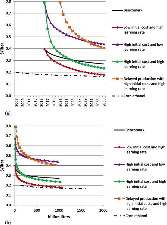
Figure 1. Effects of the biofuel mandate on processing costs of corn and cellulosic ethanol. (a) Changes in processing costs of cellulosic and corn ethanol over time. (b) Changes in processing costs of cellulosic and corn ethanol with respect to cumulative production.
Download figure:
Standard imageTable 4. Effects of the mandate on fuel mix and costs of production in 2035.
| Scenariosa | Benchmark | Scenario (1) | Scenario (2) | Scenario (3) | Scenario (4) |
|---|---|---|---|---|---|
| Fuel mix (billion liters) | |||||
| Corn ethanol | 56.8 | 56.8 | 56.8 | 56.8 | 56.8 |
| Sugarcane ethanol | 5.1 | 4.7 | 6.7 | 5.1 | 6.8 |
| Cellulosic ethanol | 89.9 | 64.0 | 101.2 | 107.8 | 103.2 |
| BTL | 13.6 | 29.0 | 2.6 | 0.0 | 1.3 |
| Biodiesel | 2.9 | 2.9 | 6.7 | 6.3 | 6.7 |
| Prices of fuels ($ per gasoline energy equivalent liter)b | |||||
| Price of gasoline | 0.90 | 0.92 | 0.92 | 0.92 | 0.92 |
| Price of diesel | 0.88 | 0.79 | 0.92 | 0.93 | 0.92 |
| Retail producer cost of corn ethanol | 1.14 | 1.14 | 1.20 | 1.18 | 1.19 |
| Industrial processing cost | 0.25 | 0.25 | 0.25 | 0.25 | 0.25 |
| (22%)c | (22%) | (21%) | (21%) | (21%) | |
| Retail producer cost of cellulosic/sugarcane ethanol | 1.29 | 1.13 | 1.54 | 1.23 | 1.45 |
| Industrial processing cost | 0.41 | 0.27 | 0.66 | 0.35 | 0.61 |
| (32%) | (24%) | (43%) | (28%) | (42%) | |
| Retail producer cost of BTL | 1.27 | 1.01 | 2.18 | 2.18 | 2.13 |
| Industrial processing cost | 0.65 | 0.41 | 1.56 | 1.56 | 1.56 |
| (51%) | (41%) | (72%) | (72%) | (73%) | |
| Biomass price ($ per MT) | 70.0 | 66.5 | 70.0 | 70.0 | 60.2 |
aScenario (1): low initial cost and high learning rates for cellulosic biofuels; scenario (2): high initial processing costs of cellulosic biofuels and low learning rate; scenario (3): high initial processing costs and high learning rates for cellulosic biofuels; scenario (4): delayed commercial production of cellulosic ethanol in addition to scenario (3). bRetail producer cost of fuels include feedstock cost, industrial processing cost, return on equity to biorefinery investors, market margin, fuel tax, transportation costs of feedstock, net of co-product credits. cNumber in parentheses represents the percentage share of unit processing cost in total biofuel production cost.
We also analyze the effects of supplementing the binding mandate with other biofuel/climate policies, including the mandate with carbon tax (mandate + carbon tax), the mandate with Low Carbon Fuel Standard (mandate + LCFS), and the mandate with the Cellulosic Biofuel Production Tax Credit (mandate + CBPTC). We compare the results to the mandate only. The carbon intensities of the various biofuels used for implementing the Low Carbon Fuel Standard are described in Chen et al (2012b, 2012c); we consider only the direct lifecycle carbon emissions here and not those due to indirect land use change (for a discussion of the conceptual and empirical reasons for not incorporating indirect land use change in biofuel policies see Khanna and Crago (2012)). Key results comparing the performance of these policies are summarized in figures 2 and 3 and table 5.
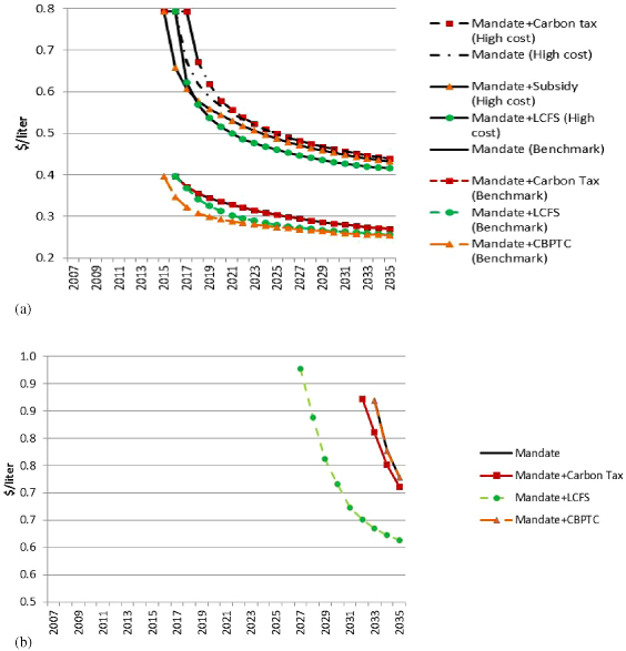
Figure 2. Effects of alternative policy combinations on processing costs of cellulosic biofuels. (a) Cellulosic ethanol. (Results with high costs of production are in the upper part of the figure.) (b) BTL with benchmark parameters.
Download figure:
Standard image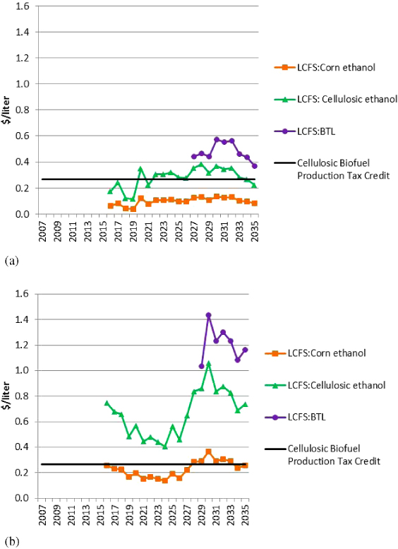
Figure 3. Subsidies for biofuels under the LCFS and the CBPTC policies. (a) Benchmark scenario. (b) High cost scenario.
Download figure:
Standard imageTable 5. Effects of supplementary policies on fuel mix and costs of biofuels in 2035.
| Scenarios | Mandate | Mandate + carbon tax | Mandate + LCFS | Mandate + CBPTC |
|---|---|---|---|---|
| Fuel mix (billion liters) | ||||
| Corn ethanol | 56.8 | 56.8 | 26.0 | 0.0 |
| Sugarcane ethanol | 5.1 | 5.3 | 4.5 | 3.6 |
| Cellulosic ethanol | 89.9 | 85.8 | 116.4 | 153.9 |
| BTL | 13.6 | 15.8 | 29.0 | 12.4 |
| Biodiesel | 2.9 | 2.9 | 1.5 | 0.4 |
| Price of fuels ($ per gasoline energy equivalent liter)a | ||||
| Price of gasoline | 0.90 | 0.98 | 0.95 | 0.89 |
| Price of diesel | 0.88 | 0.94 | 0.85 | 0.90 |
| Retail producer cost of corn ethanol | 1.14 | 1.17 | 1.09 | 0.99 |
| Industrial processing cost | 0.25 | 0.25 | 0.26 | 0.27 |
| (22%)b | (21%) | (24%) | (27%) | |
| Retail producer cost of cellulosic/sugarcane ethanol | 1.29 | 1.24 | 1.24 | 0.95 |
| Industrial processing cost | 0.41 | 0.41 | 0.39 | 0.38 |
| (32%) | (33%) | (31%) | (40%) | |
| Retail producer cost of BTL | 1.27 | 1.20 | 1.13 | 1.37 |
| Industrial processing cost | 0.65 | 0.63 | 0.55 | 0.65 |
| (51%) | (53%) | (48%) | (48%) | |
| Biomass price ($ per MT) | 70.0 | 60.4 | 63.3 | 90.0 |
aProducer prices of fuels include feedstock cost, industrial processing cost, return on equity to biorefinery investors, market margin, fuel tax, transportation costs of feedstock, net of co-product credits and subsidies. bNumbers in parentheses represent the percentages of unit processing costs in total biofuel production costs.
4.1. Effect of the mandate on processing costs of cellulosic biofuels
Figures 1(a) and (b) show the changes in unit processing costs of cellulosic ethanol with respect to time and cumulative cellulosic ethanol production, respectively. We find that by accelerating cellulosic biofuel production, the mandate stimulates learning-by-doing and leads to reductions in the unit processing costs of cellulosic ethanol by 33% from $0.40 per liter in 2015 to $0.27 per liter in 2035 with a cumulative production of 1001 BL in 2035. Due to the high costs of production, BTL diesel will not be produced until 2033 and its processing cost will be reduced by 16% from $0.87 per liter to $0.73 per liter in 2035.
However, results are sensitive to the assumptions about learning rates and initial processing costs of cellulosic biofuels. With a higher learning rate of 10% in scenario (1), unit processing costs of cellulosic ethanol decline much more quickly and its costs decrease from $0.40 per liter to $0.18 per liter making it competitive with corn ethanol (processing cost of $0.17 per liter) in 2035. Cumulative cellulosic ethanol production in this case will be 1066 BL in 2035 (the largest volume of cellulosic ethanol production across scenarios considered here), which is 6.5% higher than in the benchmark scenario. With the higher learning rates, the processing cost of BTL diesel declines by 47% to $0.46 per liter in 2035.
If the initial cost of processing cellulosic biofuels is twice as high as considered in scenario (1) then the resulting costs in 2035 are strongly dependent on the learning rates assumed. In scenario (2), with a 5% learning rate, cellulosic ethanol production will start with 0.3 BL in 2015 and cumulative production will be 970 BL in 2035, which is 3% smaller than in the benchmark. Due to the low level of learning/cumulative ethanol production, unit processing cost of cellulosic ethanol will be $0.44 per liter in 2035, highest among scenarios considered here. In contrast, in scenario (3) with a high initial cost but a high learning rate of 10%, unit processing costs of cellulosic ethanol will decrease sharply from $0.80 per liter in 2015 to $0.57 per liter in 2017 and further decline to $0.23 per liter in 2035 (this is 14% smaller than the cost in the benchmark case in 2035). Even with delayed commercial availability of cellulosic biofuels, there is a potential to reduce costs by 50% by 2035 with a high learning rate. The high costs of initial production in scenarios (2)–(4) preclude any BTL diesel production in these scenarios. Figure 1(b) shows that with high initial costs, low learning rates or delayed start-up the unit processing cost could be 50%–60% higher than the benchmark level with the same cumulative levels of production.
Table 4 summarizes the effects of the mandate on the mix of biofuels produced and their costs of production in 2035 under various assumptions about the experience curve parameters. Corn ethanol will be produced at the maximum allowed level (57 BL) in 2035 to meet the mandate. Given the nested nature of the mandate for different types of biofuels assumed here, sugarcane ethanol and cellulosic ethanol are utilized till their marginal costs of production are the same. Given the learning rates assumed here, we find sugarcane ethanol and biodiesel derived from vegetable oils play an insignificant role in meeting the mandate, together accounting for less than 8% of the total biofuels in 2035. Among the cellulosic biofuels produced, the dominant biofuel is cellulosic ethanol due to its lower cost of production compared to BTL diesel.
Across all scenarios considered here, the producer price of corn ethanol will be $1.14–$1.20 per gasoline energy equivalent liter (GEEL)5 in 2035, of which processing costs account for 21–22% ($0.25 per GEEL). Despite the significant reduction in processing costs of cellulosic biofuels, they are still an expensive alternative compared to gasoline or diesel. To induce the large amount of biomass needed for cellulosic biofuels production we find a biomass price of $60–$70 per metric ton would be needed. With this feedstock cost and the processing cost described above, the producer prices of cellulosic ethanol and BTL diesel range from $1.13–$1.54 per GEEL and $1.01–$2.18 per GEEL, respectively, in 2035. Of this, the share of industrial processing costs is 24–43% and 41–73%, respectively.
The market price of gasoline and diesel is determined endogenously in BEPAM (as described in Chen et al (2012b, 2012c)). The production of biofuels displaces gasoline and diesel and affects market prices of these fuels. Due to the differences in the mix of biofuels, the extent to which gasoline and diesel are displaced differs across the scenarios examined. This has implications for the gasoline and diesel prices in 2035. We find that the price of gasoline ranges from $0.9–$0.92 per GEEL and of diesel from $0.79–0.93 per GEEL in 2035. This implies that on an energy equivalent basis, cellulosic ethanol will be 23%–67% more expensive than gasoline in 2035 depending on the initial costs and learning rates. We find that with high initial costs, cellulosic ethanol will be 34% more expensive than energy equivalent gasoline if a 10% learning rate is achieved but 67% more expensive if a 5% learning rate is achieved. Figures 1(a) and (b) suggest that the projected costs of biofuels in 2035 are more sensitive to the speed with which learning occurs and less sensitive to uncertainty in the initial production cost.
4.2. Effects of supplementary policies on costs of biofuel production
Figures 2(a) and (b) show the processing cost reductions of cellulosic biofuels under various biofuel/climate policies under two alternative assumptions about initial processing costs. We find that in the benchmark case supplementing the biofuel mandate with a carbon tax of $30 per metric ton of CO2 will not lead to a significant difference in the mix of biofuels produced and in the reduction in future processing costs of cellulosic ethanol compared to the mandate alone. In contrast, the addition of a Low Carbon Fuel Standard or the Cellulosic Biofuel Production Tax Credit to the mandate will significantly increase the incentives to produce cellulosic biofuels compared to corn ethanol and sugarcane ethanol; the addition of these policies increases the volume of cellulosic biofuels produced and leads to a larger reduction in processing costs of cellulosic ethanol than under the mandate alone, as shown in figure 2(a). When the initial costs are high, the addition of a carbon tax reduces fuel consumption but does not induce additional cellulosic biofuel production beyond the mandate. As a result it reduces the learning-based cost reductions that would be achieved by the mandate alone. The Low Carbon Fuel Standard now induces greater learning than the production tax credit for reasons discussed below.
The addition of a Low Carbon Fuel Standard to the mandate also leads to a reduction in processing costs of BTL diesel beyond those under the mandate also (see figure 2(b)); this is due to the large implicit subsidies it provides. In contrast, the production tax credit has no additional impact beyond the mandate in inducing BTL diesel production because it is not large enough to induce BTL diesel production.
Figures 3(a) and (b) display the implicit subsidies provided to corn and cellulosic ethanol and BTL under the mandate + LCFS scenario and the explicit subsidy under the mandate + CBPTC scenario. The implicit subsidy in the case of the mandate + LCFS policy is the additional incentive needed beyond that under the mandate to induce biofuel production to meet the intensity standard. The magnitude of the implicit subsidy is inversely related to the carbon intensity of the biofuel relative to the carbon intensity standard and the stringency of the intensity standard. The subsidy increases as the Low Carbon Fuel Standard becomes increasingly stringent; however the increase is not monotonic. This is because the mandate is also increasing over time and resulting in higher levels of cellulosic biofuel production. This reduces the additional amount of biofuel required to meet the Low Carbon Fuel Standard beyond that produced to meet the mandate. Moreover, as the intensity standard becomes more stringent the gap between the standard and the carbon intensity of biofuels decreases; this also tends to decrease the level of subsidies. The implicit subsidy for corn ethanol ranges from $0.04 to $0.13 per liter and for cellulosic ethanol from $0.12 to $0.38 per liter. The implicit subsidy for BTL diesel is positive from 2027 onwards and ranges from $0.37 to $0.57 per liter. In contrast, the Cellulosic Biofuel Production Tax Credit provides a uniform incentive over time ($0.27 per liter) which is larger than that under the Low Carbon Fuel Standard for cellulosic biofuels in the early years and lower in the later years. As a result, the Cellulosic Biofuel Production Tax Credit induces a larger volume of cellulosic biofuel production in the early years compared to the Low Carbon Fuel Standard. The Low Carbon Fuel Standard incentivizes more BTL production than the Cellulosic Biofuel Production Tax Credit, because it provides a higher implicit subsidy, and leads to a greater reduction in processing costs of BTL. Nevertheless, supplementing the mandate with either of these two policies could result in the achievement of the same level of costs 7–9 years earlier than under the mandate alone.
If initial costs are relatively high, the Cellulosic Biofuel Production Tax Credit is not sufficient in the long run to sustain incentives for additional production beyond the level under the mandate, as shown in figure 2(a). As a result, in 2035, processing costs of cellulosic ethanol under the mandate + CBPTC policy are similar to those under the mandate alone. With the high costs of production, the implicit subsidy to cellulosic ethanol under the Low Carbon Fuel Standard is significantly higher than in the benchmark case and ranges from $0.44 to 1.06 per liter of ethanol over the 2015–35 period (see figure 3(b)). The production of cellulosic ethanol under the mandate + LCFS starts one year later than with the Cellulosic Biofuel Production Tax Credit, but production volumes are subsequently higher under the mandate + LCFS scenario; as a result the latter policy leads to a larger reduction in processing costs than the mandate + CBPTC. Moreover, even with high initial costs of production of cellulosic ethanol, the mandate + LCFS achieve the same processing costs as those under the mandate scenario in 2035, by 2028. On the other hand, the mandate + CBPTC achieves this reduction in processing costs by 2033 (see figure 2(a)). Figure 2(b) shows that cost reductions in BTL start sooner and are much larger when a mandate is combined with a Low Carbon Fuel Standard. The addition of the production tax credit to the mandate does not incentivize additional production of BTL diesel and its processing costs remain similar to those under the mandate alone, with production becoming viable after 2033.
Table 5 shows that the mix of biofuels induced under the mandate with a carbon tax is not considerably different than those under the mandate alone. Adding the Low Carbon Fuel Standard to the mandate will lead to a total amount of 166 BL of cellulosic biofuel production in 2035 (primarily in the form of cellulosic ethanol); this volume is even higher under the mandate + CBPTC (175 BL) with consequent reductions in the amount of corn ethanol produced. The mandate + LCFS also induces larger volumes of BTL diesel than the mandate alone due to the value it places on reduction in GHG intensity per unit energy. In contrast, Cellulosic Biofuel Production Tax Credit does not reward the higher energy content of BTL and shifts the mix of cellulosic biofuels towards ethanol instead of BTL. The demand for biomass is also larger with these supplementary policies and the biomass price increases to $90 per MT under the mandate + LCFS scenario in 2035.
The addition of the carbon tax, Low Carbon Fuel Standard or Cellulosic Biofuel Production Tax Credit lowers the gap between the retail price of cellulosic ethanol and energy equivalent price of gasoline. Under the mandate, cellulosic biofuels will be 40% more expensive than energy equivalent gasoline in 2035. The addition of the Low Carbon Fuel Standard or the carbon tax would reduce the retail costs of cellulosic biofuels so that they are 30% more expensive than energy equivalent gasoline. The mandate + CBPTC lowers the cost gap to be only 7% in 2035.
BTL diesel, on the other hand, is about 44% more expensive than energy equivalent diesel under the mandate in the benchmark case. The direction of the effect of supplementary policies on costs of BTL diesel differs across policies. While the addition of a carbon tax and a Low Carbon Fuel Standard stimulate additional production of BTL diesel and lower their costs so that they are now 30% more expensive than energy equivalent diesel in 2035, the Cellulosic Biofuel Production Tax Credit will result in higher costs of BTL (making them over 50% more expensive than energy equivalent diesel) than under the benchmark assumptions. This is because the Cellulosic Biofuel Production Tax Credit increases incentives to produce cellulosic ethanol instead of BTL diesel.
5. Conclusions
This letter examines the extent to which targeted levels of biofuel production can be anticipated to lead to a reduction in production costs of cellulosic biofuels due to learning-by-doing under various assumptions about initial processing costs, learning rates and timing of commercial production. We also explore the effect of supplementary policies in stimulating reductions in the processing costs of biofuels by accelerating production beyond the minimum levels mandated. Biofuel/climate policies differ in the type of biofuels they will incentivize and the path of learning-by-doing they induce. We analyze their effects under various assumptions about initial processing costs and learning rates.
Assuming learning rates of 5%–10% for cellulosic biofuels, we find that binding biofuel targets can reduce the processing cost of cellulosic ethanol by about 30%–70% between 2015 and 2035. We also find that policies can affect the rate of adoption and cost reductions over time. The addition of supplementary policies that provide greater incentives for cellulosic biofuels than the mandate alone can achieve similar reductions in these costs several years earlier than the mandate alone. Despite these policies, however, cellulosic biofuels will still be considerably more expensive than liquid fossil fuels in 2035, given the learning rates assumed here. This implies that they will require continued policy incentives in order to continue to induce their production and consumption. Higher learning rates than those assumed here will be needed to accelerate the reduction in these processing costs and make them competitive with first-generation biofuels and fossil fuels earlier than 2035. The timing and magnitude of the cost reductions are expected to be sensitive to a number of other factors that affect market penetration rates of biofuels, including the elasticity of supply of gasoline and diesel, the costs of feedstock production, and the demand for vehicle kilometers travelled with alternative types of vehicles.
The presence of learning-by-doing suggests that increased production by a refinery will reduce production costs for the entire industry by increasing the cumulative production experience of the industry. These knowledge spillovers would lead to a market failure and under-production of biofuels if refineries cannot appropriate the social benefits of the additional biofuel production; thus the presence of the knowledge spillovers justifies government intervention in the biofuel industry. Although our analysis does not examine the design of optimal policy given the learning rates assumed here it does show that effective policy designs can play an important role in stimulating cost-reducing innovations in the biofuel industry. Our analysis also assumed that the learning rate remains the same across various policies and over time. Further research is needed to understand how policy drives innovation and the learning process.
Acknowledgments
Senior authorship is not assigned. Funding from the Energy Biosciences Institute, University of California, Berkeley, is gratefully acknowledged.
Footnotes
- 4
- 5