
Abstract
The Sun has surely been a major external forcing to the climate system throughout the Holocene. Nevertheless, opposite trends in solar radiation and temperatures have been empirically identified in the last few decades. Here, by means of an inferential method—the Granger causality analysis—we analyze this situation and, for the first time, show that an evident causal decoupling between total solar irradiance and global temperature has appeared since the 1960s.
Export citation and abstract BibTeX RIS

Content from this work may be used under the terms of the Creative Commons Attribution-NonCommercial-ShareAlike 3.0 licence. Any further distribution of this work must maintain attribution to the author(s) and the title of the work, journal citation and DOI.
1. Introduction
A number of studies have indicated the major role of the Sun in contributing to drive climate throughout the Holocene: see, for instance, Jansen et al (2007) and references therein. Recently, however, by simple correlation and graphical methods it has been found that solar radiation shows an evidently contrary behavior compared with the temperature trend since the 1980s (Lockwood and Fröhlich 2007, Stauning 2011).
Thus, it seems that there has been a decoupling between solar forcing and recent temperature behavior. Then, we could ask: is this decoupling a causal one? And, if it proves to be a causal decoupling, is it possible to put a date on the loss of importance of solar influences on temperature? Here, we address these problems by an inferential method, through a Granger causality analysis.
Recently, this method has been applied to specific causality problems in the climate system (Diks and Mudelsee 2000, Kaufmann et al 2003, Elsner 2006, 2007, Mosedale et al 2006, Kaufmann et al 2007, Mohkov et al 2011) and to the topic of climatic attribution (Sun and Wang 1996, Kaufmann and Stern 1997, Reichel et al 2001, Triacca 2001, 2005, Mohkov and Smirnov 2008, Kodra et al 2011, Attanasio et al 2012).
The notion of Granger causality is quite simple. Suppose that we have three variables: y,x and z, and that we first attempt to forecast yt+1 using past values of y and z. We then try to forecast yt+1 using past values of y,x and z. We say that x Granger causes y if the latter forecast is found to be more successful, according to the calculated values of mean square error (MSE). Here y is global temperature (T), z is an index of natural variability and x is total solar irradiance (TSI) or greenhouse gases total (CO2+CH4+N2O) radiative forcing (GHG).
The notion of Granger causality did not mention anything about possible instantaneous correlation between x and y, the so-called instantaneous causality. Here, we will not test for instantaneous causality because it does not say anything about the cause and effect relation (see Lütkepohl 2005).
In a previous paper (Attanasio et al 2012), we considered bivariate analyses between natural or anthropogenic forcings and global temperature, and found GHG Granger causality effects on temperature since the 1940s, while TSI and other natural forcings do not Granger-cause temperature in the same period. Here, due to the evidence that natural variability affects temperature behavior on decadal time scales—see, for instance, DelSole et al (2011) and Wu et al (2011)—we extend our information set to one of the indices of the Pacific Decadal Oscillation (PDO), the Atlantic Multidecadal Oscillation (AMO) or El Niño Southern Oscillation (ENSO). As is well known, a trivariate extension gives to the Granger technique a better reliability with respect to a bivariate analysis (see, for instance, Lütkepohl 1982).
In this paper the recent climatic role of the Sun is investigated in this trivariate framework.
2. Data
Time series of mean annual data since the middle of the 19th century to 2007 are considered for the following variables:
- HadCRUT3 combined global land and marine surface temperature anomalies (Brohan et al 2006): data available at www.cru.uea.ac.uk/cru/data/ (since 1850);
- TSI (Lean and Rind 2008), with background from Wang et al (2005): data available at www.geo-fu.berlin.de (since 1850);
- CO2, CH4 and N2O concentrations (Hansen et al 2007): data available at http://data.giss.nasa.gov (since 1850); greenhouses gases total (CO2+CH4+N2O) radiative forcing (GHG) has been calculated as in Ramaswamy et al (2001);
- Southern Oscillation Index (SOI), related to ENSO (Ropelewski and Jones 1987, Allan et al 1991, Können et al 1998): data available at www.cru.uea.ac.uk/cru/data/soi/soi.dat (since 1866);
- Pacific Decadal Oscillation (PDO) (Smith and Reynolds 2004): data available at ftp.ncdc.noaa.gov/pub/data/ersst-v2/pdo.1854.latest.st (since 1854);
- Atlantic Multidecadal Oscillation (AMO) (Enfield et al 2001): data available at www.esrl.noaa.gov/psd/data/timeseries/AMO (since 1856).
3. Method
The climate system is nonlinear and applying linear methods for climatic analyses of causal links could seem inappropriate. Actually, if annual averages are considered, as in our case, it is quite reasonable that as a consequence of the central limit theorem (Yuval and Hsieh 2002), averaging can produce near-linear climate relations among variables of the climate system, even if it is necessary to deal with nonlinear relationships at shorter temporal and smaller spatial scales. Thus, we are confident that a linear analysis, such as Granger's, can provide a 'first-order' estimate of the existence or non-existence of causal links in the climate system.
The notion of Granger causality was first introduced by Wiener (1956) and later reformulated by Granger (1969). For our application, we assume that a trivariate time series  follows a vector autoregression (VAR) model of finite order k:
where c = (c1,c2,c3) is a vector of constants, ϕil,j are fixed coefficients and (u1t,u2t,u3t) is a trivariate white noise process. The model order k is kept low (k = 1,...,4)—in doing so the models are parsimonious—and the models finally selected are those endowed with the best predictive performance on each test set, choosing for k the following value:
where PC(k) = ln[det(Σk)] and Σk is the covariance matrix evaluated on the residuals of the test set.
In this framework, in order to test the null hypothesis of non-causality

we use an out-of-sample Granger causality test. The sample of observations  is divided into a training part and a test part. The test part is represented by the last P observations, while the training sample consists of all the previous R = N − P observations. We then consider the unrestricted model (1) and the following restricted model:
Using the training set, the parameters of the model are estimated by estimated generalized least squares (EGLS) and the P one-step-ahead forecast errors for t = R + 1,...,R + P are calculated as:
Here we use a fixed scheme for calculation of our forecasts, i.e. each one-step-ahead forecast is generated using parameters that are estimated only once employing data from 1 to R. Then we evaluate the mean square prediction errors on test sets defined as:
In order to test the null hypothesis

versus

we use two tests described in McCracken (2007) and Attanasio et al (2012)—see these references for further details: the MSE-t test, commonly attributed to Diebold and Mariano (1995) or West (1996), and the MSE-REG test, suggested by Granger and Newbold (1977). Here, we use both tests in order to evaluate the robustness of the results. In our case, however, we do not use the critical values described in McCracken (2007) because our time series are not stationary. Thus, the critical values of the tests are calculated by means of the following bootstrap method (bootstrap based on residuals).
- (1)
- (2)Evaluate MSE-t and MSE-REG statistics.
- (3)Under the null hypothesis of non-causality, estimate the restricted model (2) employing the full sample and extract the estimates
 and the residuals .
 - (4)Apply the bootstrap procedure (resampling with replacement) on and obtain the pseudo-residuals .
- (5)Create the pseudo-data given by
- (6)Using these pseudo-data, repeat steps 1 and 2, calculating MSE-t and MSE-REG bootstrap statistics.
- (7)Repeat steps from 4 to 6 M times (in our application M = 10 000; this value guarantees the convergence of p-values).
- (8)Calculate the bootstrap p-values.


We are aware that Granger causality is just one of the possible definitions of causality. However, since Granger causality is based on precedence and predictability, it can represent a helpful tool identifying the direction of causation.
4. Results
In this framework, we test the null-hypotheses of Granger non-causality from TSI or GHG to T. Data sets span from the middle of the 19th century to 2007. We perform out-of-sample tests on five test sets which span the following periods: 1941–2007, 1951–2007, 1961–2007, 1971–2007, 1981–2007. As already cited, a fixed scheme is adopted for predictions, and the statistical significance of results is evaluated by MSE-t and MSE-REG tests.
In order to test if the residuals of our unrestricted VAR models can be considered a realization of a multivariate white noise, we use the portmanteau test for autocorrelation and the multivariate ARCH-LM test for homoskedasticity (constant variance with time), as described in Lütkepohl (2005). The results of these tests are presented in tables 1 and 2. We stress that the residuals of our models are uncorrelated and homoskedastic, as required for the correct application of our bootstrap procedure. In addition, analogous univariate tests for autocorrelation (Ljung–Box test) and ARCH tests for homoskedasticity have also been applied to single residual series. The results do not change with respect to those of the multivariate tests.
Table 1. Results of tests of autocorrelation and homoskedasticity for x = GHG. The null hypothesis is non-autocorrelation for the portmanteau test and homoskedasticity for the ARCH-LM test. The maximum lag in the portmanteau test is chosen as the 20% of training observations (number in parenthesis). For the ARCH-LM the maximum lag is chosen equal to 5.
| x,z | Training set | VAR order | p-value portmanteau test | p-value ARCH-LM test |
|---|---|---|---|---|
| GHG | 1854–1940 | 2 | 0.7242 (17) | 0.2370 |
| PDO | 1854–1950 | 2 | 0.3589 (19) | 0.2215 |
| 1854–1960 | 2 | 0.2441 (21) | 0.3096 | |
| 1854–1970 | 2 | 0.7235 (23) | 0.3757 | |
| 1854–1980 | 2 | 0.6421 (25) | 0.1337 | |
| GHG | 1866–1940 | 2 | 0.4345 (15) | 0.2078 |
| ENSO | 1866–1950 | 2 | 0.2663 (17) | 0.2662 |
| 1866–1960 | 2 | 0.1858 (19) | 0.2471 | |
| 1866–1970 | 2 | 0.6381 (21) | 0.0743 | |
| 1866–1980 | 2 | 0.8390 (23) | 0.0178 | |
| GHG | 1856–1940 | 2 | 0.9473 (17) | 0.5299 |
| AMO | 1856–1950 | 2 | 0.7914 (19) | 0.4043 |
| 1856–1960 | 2 | 0.7907 (21) | 0.3422 | |
| 1856–1970 | 2 | 0.9754 (23) | 0.4712 | |
| 1856–1980 | 2 | 0.9715 (25) | 0.0997 |
Table 2. As in table 1, but for x = TSI.
| x,z | Training set | VAR order | p-value portmanteau test | p-value ARCH-LM test |
|---|---|---|---|---|
| TSI | 1854–1940 | 2 | 0.8371 (17) | 0.1238 |
| PDO | 1854–1950 | 2 | 0.8371 (19) | 0.0798 |
| 1854–1960 | 3 | 0.6208 (21) | 0.1297 | |
| 1854–1970 | 3 | 0.4885 (23) | 0.1952 | |
| 1854–1980 | 2 | 0.0890 (25) | 0.1323 | |
| TSI | 1866–1940 | 2 | 0.7742 (15) | 0.2593 |
| ENSO | 1866–1950 | 2 | 0.5518 (17) | 0.2252 |
| 1866–1960 | 2 | 0.6932 (19) | 0.2838 | |
| 1866–1970 | 2 | 0.5107 (21) | 0.2931 | |
| 1866–1980 | 2 | 0.3424 (23) | 0.2541 | |
| TSI | 1856–1940 | 2 | 0.9425 (17) | 0.6178 |
| AMO | 1856–1950 | 2 | 0.8188 (19) | 0.6312 |
| 1856–1960 | 2 | 0.9198 (21) | 0.4879 | |
| 1856–1970 | 2 | 0.8450 (23) | 0.3852 | |
| 1856–1980 | 2 | 0.7738 (25) | 0.2662 |
The first result of our Granger analysis is very clear: if we take GHG as the x variable, in every case (all circulation patterns and test sets considered)—except one—the null hypothesis of Granger non-causality on T is rejected at the 5% significance level, and very often also at 1% significance. This is clear evidence that there is a causal link (in the Granger sense) between GHG and global temperature since 1941 up to the present day: see table 3 for detailed results.
Table 3. Results of Granger causality significance tests for x = GHG. A non-significant (ns) statistics implies that the null hypothesis of Granger non-causality cannot be rejected at 5% significance level, while * and ** indicate that the null hypothesis is rejected at the 1% and 5% significance level, respectively. VAR orders are the k values for the models with the best predictive ability.
| x,z | Test set | VAR order | MSE-tp-value | VAR order | MSE-REG p-value |
|---|---|---|---|---|---|
| GHG | 1941–2007 | 2 | 0.0076* | 2 | 0.0051* |
| PDO | 1951–2007 | 2 | 0.0162** | 2 | 0.0099* |
| 1961–2007 | 2 | 0.0073* | 2 | 0.0036* | |
| 1971–2007 | 2 | 0.0041* | 2 | 0.0014* | |
| 1981–2007 | 2 | 0.0081* | 2 | 0.0049* | |
| GHG | 1941–2007 | 2 | 0.0146** | 2 | 0.0119** |
| ENSO | 1951–2007 | 2 | 0.0382** | 2 | 0.0336** |
| 1961–2007 | 2 | 0.0093* | 2 | 0.0046* | |
| 1971–2007 | 2 | 0.0053* | 2 | 0.0030* | |
| 1981–2007 | 2 | 0.0080* | 2 | 0.0053* | |
| GHG | 1941–2007 | 2 | 0.0358** | 2 | 0.0261** |
| AMO | 1951–2007 | 2 | 0.1462 ns | 2 | 0.1449 ns |
| 1961–2007 | 2 | 0.0553 ns | 2 | 0.0423** | |
| 1971–2007 | 2 | 0.0148** | 2 | 0.0046* | |
| 1981–2007 | 2 | 0.0103** | 2 | 0.0042* |
Vice versa, if TSI is considered as the x variable, a Granger causal link is significant only in the first test set when AMO is included in the information set, and in the first two sets when PDO and ENSO are considered. In more recent periods this causal link disappears: see table 4 for specific results.
Table 4. Results of Granger causality significance tests for x = TSI. A non-significant (ns) statistics implies that the null hypothesis of Granger non-causality cannot be rejected at the 5% significance level, while * and ** indicate that the null hypothesis is rejected at 1% and 5% significance levels, respectively. VAR orders are the k values for the models with the best predictive ability.
| x,z | Test set | VAR order | MSE-tp-value | VAR order | MSE-REG p-value |
|---|---|---|---|---|---|
| TSI | 1941–2007 | 2 | 0.0013* | 2 | 0.0023* |
| PDO | 1951–2007 | 2 | 0.0104** | 2 | 0.0195** |
| 1961–2007 | 3 | 0.0521 ns | 3 | 0.0581 ns | |
| 1971–2007 | 3 | 0.3961 ns | 3 | 0.3988 ns | |
| 1981–2007 | 2 | 0.6992 ns | 2 | 0.7202 ns | |
| TSI | 1941–2007 | 2 | 0.0021* | 2 | 0.0044* |
| ENSO | 1951–2007 | 2 | 0.0266** | 2 | 0.0400** |
| 1961–2007 | 2 | 0.1339 ns | 2 | 0.1282 ns | |
| 1971–2007 | 2 | 0.5018 ns | 2 | 0.5122 ns | |
| 1981–2007 | 2 | 0.8494 ns | 2 | 0.8774 ns | |
| TSI | 1941–2007 | 2 | 0.0042* | 2 | 0.0063* |
| AMO | 1951–2007 | 2 | 0.1862 ns | 2 | 0.1932 ns |
| 1961–2007 | 2 | 0.5217 ns | 2 | 0.5607 ns | |
| 1971–2007 | 2 | 0.844 ns | 2 | 0.8951 ns | |
| 1981–2007 | 2 | 0.8665 ns | 2 | 0.9079 ns |
The situation becomes even clearer if the p-values of tests are plotted for every test period, as in figure 1. These pictures show that, while the influence of GHG on global temperature remains important throughout all the periods, the Granger causal link between TSI and T becomes progressively less evident with time and completely disappears for the last two periods. In particular, the influences of GHG and TSI on T appear comparable until the 1950s, but, after that decade, a clear causal decoupling between TSI and T is evident and very marked in the data of our Granger analysis. At the same time, the Granger causality from GHG to T remains robust and, possibly, becomes even more evident: the p-values, which are already very small, decrease further.
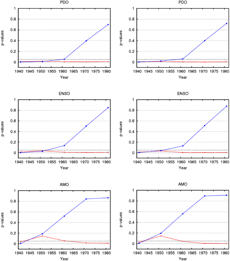
Figure 1. Plot of the p-values from the MSE-t (left) and MSE-REG (right) tests when x = TSI (blue line) and x = GHG (red line) for the different variables z = circulation patterns. The significance threshold of 0.05 is shown (dashed line). The increase in p-values over the recent decades is evident for the performance of the model with TSI.
Download figure:
Standard imageAs a final remark, it is worthwhile noting that the p-values of the Granger causality tests when AMO is considered in the information set are always higher than the corresponding ones in the cases of z = PDO, ENSO. Thus, when AMO is inserted in the information set, the causal role of external forcings seems to weaken (see also figure 1). This indirectly suggests that, among the various patterns of natural variability, AMO plays a more relevant role in driving the global temperature behavior at decadal time scales.
5. Conclusions
We have shown that there is an evident causal decoupling between total solar irradiance and global temperature in recent periods. Our work permits us to fix the 1960s as the time of the loss of importance of solar influence on temperature. At the same time greenhouse gases total radiative forcing has shown a strong Granger causal link with temperature since the 1940s up to the present day.
Our results obviously suggest the need for further research to investigate in greater depth the causes of this Sun-temperature decoupling, but, at the same time, they appear as a clear contribution to the debate on the causes of recent global warming.