Branchfall dominates annual carbon flux across lowland Amazonian forests

David C Marvin; Gregory P Asner

doi:10.1088/1748-9326/11/9/094027

Introduction

Tropical forests play an important role in constraining atmospheric CO₂ concentrations. As the largest terrestrial carbon sink in the world, tropical forests are estimated to trap and store more than 1.19 ± 0.41 Pg carbon per year—equivalent to the annual emissions of the European Union (Boden et al 2010)—that would otherwise remain in the atmosphere as heat-trapping CO₂ (Pan et al 2011). While ecologists are gaining ever-improving global information on tropical forest carbon stocks (Baccini et al 2012, Avitabile et al 2016), sub-continental estimates are still highly uncertain (Baccini and Asner 2013, Mitchard et al 2013, Sexton et al 2015). Accurately estimating changes over time in tropical forest aboveground carbon stocks (or carbon density, aboveground carbon density (ACD)) at sub-continental scales is crucial for understanding the ecological and functional roles of these forests in a global context.

While carbon emissions resulting from tropical deforestation are better resolved (Harris et al 2012), carbon fluxes from intact forests are just as important but remain poorly understood. Multiple studies report a net carbon sink in the tropics based on evidence from repeated censuses of forest plots, remote sensing observations, atmospheric inverse modeling, and eddy flux towers (table S1). However, all of these estimates are highly uncertain and subject to considerable debate (Chambers et al 2009, 2013, Gloor et al 2012). Current estimates range from marginal sink values near zero to substantial sink values of up to 0.94 Mg C ha⁻¹ yr⁻¹, with some reporting a carbon source in individual years. There are myriad causes for the high uncertainty surrounding estimates of ACD fluxes (Marvin et al 2014), but a fundamental source of this uncertainty stems from the lack of large-scale, high-spatial resolution multi-temporal data.

Although rarely quantified, branchfall is an important ecological process that, when measured, can improve estimates of ecosystem processes. Tree crowns in tropical forests comprise approximately one-quarter to one-half of the total aboveground woody biomass (e.g., Higuchi et al 1998, Malhi et al 1999, Goodman et al 2014). As these crowns fragment over time they form an important biogeochemical flux, returning both carbon and nutrients to the soil beyond the standard flux from leaf litterfall or whole tree mortality. While branchfall and partial crown failures (i.e., non-fatal tree damage) are not generally considered a meaningful part of gap dynamics, they are sometimes measured as part of plot necromass surveys (e.g., Palace et al 2008, Doughty et al 2015, Malhi et al 2015), and are assumed to be implicitly captured over long time scales as a result of standard allometric scaling techniques. The ability to explicitly quantify and map branchfall (and tree mortality) over large areas will allow more accurate estimates of ecosystem carbon and nutrient flux by reducing uncertainties related to tree allometry and mortality (Palace et al 2008) and spatial upscaling from field plots/transects (Chambers et al 2013, Marvin et al 2014).

Understanding changes in branchfall and structural damage over time also provides ecologically important insights. Drought and other climate events (van der Meer and Bongers 1996, Doughty et al 2015), disease/pests, and mechanical stress from lianas and epiphytes (Putz 1984) are a few mechanisms that affect the rate of branchfall and other non-fatal tree damage. The resulting necromass produced by branchfall and tree mortality, as well as the increased light availability, creates structural habitat for a variety of organisms (e.g., Schemske and Brokaw 1981, Svenning 2000, Mac Nally et al 2001). Moreover, branchfall plays an important role in forest productivity (Chambers et al 2001), seedling/sapling regeneration and growth (Denslow 1987, Clark and Clark 1991), and nutrient cycling (Vitousek and Sanford 1986). A lack of branchfall data restricts the ability of ecologists to better understand and predict many ecosystem processes.

Here we examine 12 widely distributed landscapes totaling nearly 100 000 ha of lowland western Amazonian forest from a repeat airborne light detection and ranging (LiDAR) campaign (figure 1(A); table S2). We quantify full tree mortality (full canopy gaps, figure 1(D)), branch-and partial crownfall (upper canopy gaps, figure 1(E)) at 2 m spatial resolution, and calculate the estimated gross carbon source to the atmosphere of each gap type at 1 ha spatial resolution. No study has explicitly measured and incorporated branchfall as part of aboveground gross carbon losses at the landscape scale (10³–10⁵ ha), due to the difficulty of quantifying branchfall using field surveys (Clark et al 2001a). We emphasize our measurement of gross rather than net carbon flux, with gross flux estimates (and gap formation rates generally) more pertinent to full accounting of tropical forest carbon dynamics. This study (1) investigates the difference between branchfall and tree mortality in western Amazon landscapes, (2) uncovers regional variation in gap dynamics, and (3) explores the potential for high-resolution measurement of gap dynamics to improve estimates of ecosystem processes.

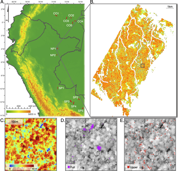
**Figure 1.** Overview of study area and gap types. (A) Map of landscapes (1:1 scale) in Colombia and Peru used in the analysis. (B) Map of top-of-canopy height (TCH) for a single landscape (NP1) with inscribed square corresponding to zoom boxes containing 2-D raster images of colored TCH with static gaps in dark blue (C), greyscale TCH with dynamic full canopy gaps in purple (D), and greyscale TCH with dynamic upper canopy gaps in red (E). Coloring in (B) is same as in (C), and spatial scaling in (D) and (E) is the same as in (C).
Download figure:
Standard image High-resolution image

Methods

Study landscapes

We selected 12 landscapes distributed across a 1600 km longitudinal gradient of lowland tropical forests from northwest to southwest Amazonia (figure 1(A); table S2). Across all the landscapes, elevations ranged from 135 to 402 m above sea level (2 m resolution LiDAR digital terrain model (DTM), see below), mean annual precipitation (Huffman et al 2007) ranged from 1951 to 3492 mm (∼25 km resolution), and mean annual temperature (Hijmans et al 2005) ranged from 24.3 to 26.7 °C (∼5 km resolution). The geology of the landscapes is erosional terra firme substrate on elevated terraces, depositional floodplain substrate in low-lying areas near rivers and streams, or a mix of both. Dominant soil types (FAO-UNESCO 2005) in each landscape were Oxisols and Ultisols. These landscapes were chosen to be outside the main areas of the 2010 Amazon basin drought. The 2010 drought extended into the central Peruvian Amazon but was not extensive enough to affect the chosen landscapes mostly in the far SW and NE areas of Peru (Lewis et al 2011, Saatchi et al 2013). For each landscape we calculated mean dry-season (July–September) standardized precipitation evapotranspiration index (SPEI) (Vicente Serrano et al 2010) values extracted from SPEIbase (Beguería et al 2010) (table S2). None of the landscapes have a 2010 SPEI value below −1, which is considered to be the threshold for drought (Mitchell et al 2014).

Airborne LiDAR collection and processing

Depending on the landscape, LiDAR data were either collected in 2011 and 2012, or 2011 and 2013 (table S2) using the Carnegie Airborne Observatory-2 (CAO) Airborne Taxonomic Mapping System (AToMS), which is carried onboard a Dornier 228 aircraft (Asner et al 2012). The AToMS LiDAR is a dual laser, scanning waveform system capable of operating at 500 000 laser shots per second. For the data collection, the aircraft was operated at speeds of up to 110 knots at an altitude averaging 2000 m above ground level. The LiDAR settings were maintained to sample a mean on-the-ground laser spot spacing of 2 shots m⁻², peaking at 4 shots m⁻² in areas of flightline overlap. This level of sampling ensured that the derived LiDAR measurements were highly precise in horizontal and vertical space (Asner et al 2012), with a combined between-flight uncertainty for top-of-canopy returns of ±17.0 cm horizontally and ±15.6 cm vertically for these flights.

Following data acquisition, laser ranges from the LiDAR were combined with embedded high resolution Global Positioning System-Inertial Measurement Unit data to determine the 3D locations of laser returns, producing a 'cloud' of LiDAR data (figure 2). A DTM, digital surface model, and top-of-canopy height (TCH) layer were produced for each landscape and for each year. We masked out non-forested areas, water bodies, and other anomalous landscape features. Each resulting landscape has at least 1900 ha of sampling area, with a total sampled area of 97 780 ha. See SI methods for more detail on the airborne LiDAR collection and processing.

**Figure 2.** LiDAR 3-D point cloud from example area in landscape NP1 showing dynamic gaps. (A) LiDAR derived top-of-canopy height map at 2 m resolution with coloring as in Fig. 1C. (B) Top view of LiDAR three-dimensional point cloud with full (purple) and upper (yellow) canopy gaps, and (C) isometric view of (B). (D) Zoom inset from (B) and (C) showing an isometric view of a large full canopy and multiple smaller upper canopy gaps. In (B-D) the green colored points are year 2 data, while gap colored points (purple and yellow) are points that were present in year 1 but were not present in year 2. Gray points are those present in year 1 no longer present in year 2 but did not meet the dynamic gap criterion (see Methods).
Download figure:
Standard image High-resolution image

Canopy gap determination

Traditionally studies of gap dynamics employ the gap definition developed by Brokaw (1982), or a slight modification thereof, who defined a canopy gap as an opening 'in the forest canopy extending through all levels down to an average height of two m above ground'. We find this definition to be overly simplistic and unfit for landscape-scale studies of gap dynamics using LiDAR-derived TCH data. Instead we define gaps based on the difference in relative height from the surrounding canopy. For each TCH layer, we created a TCH_mean layer using a mean smoothing filter with a one ha kernel. The TCH_mean was subtracted from the original TCH layer, and divided by TCH_mean to produce a relative TCH layer. For all classified gap types (see below) we computed the gap size-frequency variable λ for static full, dynamic full, and dynamic upper canopy gaps. We used the approach and R syntax provided by Asner et al (2013) and described in more detail by Marvin et al (2014). We calculated the gap density (gaps ha⁻¹) and the mean gap size per unit area for all gap types.

Static and dynamic full canopy gaps

Static gaps (those present only at a single time period) were classified as having a relative TCH of −0.7 to −1.0, or 70%–100% below the mean forest height of the surrounding 1 ha at each data collection time period. This allows identification of gaps over short timescales (1–2 years) using airborne LiDAR even when tree fall debris, understory shrubs or small trees, and/or rapidly growing pioneer species fill in the full canopy gap above the 2 m Brokaw threshold. Other thresholds considered yielded similar results (Asner et al 2013).

Using the final static gap layers from the two sampling years, we classified dynamic full gaps (those newly formed during the sampling period) as only those pixels that were not classified as a static gap in Year 1, but met the static gap definition above in Year 2. To reduce gap false positives, only three or more contiguous pixels (areas ≥ 12 m²) were retained as static or dynamic full canopy gaps.

Dynamic upper canopy gaps

We refine and extend the concept of upper canopy gaps to be applicable to dynamic measurements of forest gaps. Dynamic upper canopy gaps are newly formed gaps during the sampling period resulting from medium-to-large branch falls and partial crown failures of trees that form the canopy layer of an intact forest. These gaps are isolated to the canopy layer and do not extend to the ground. For each landscape, Year 1 TCH was subtracted from Year 2 TCH, and divided by Year 1 TCH to produce the relative TCH change between the two sampling periods. We define dynamic upper canopy gaps as a relative loss in canopy height between the two sampling periods of 0.1–0.4, or a 10%–40% height loss below the mean forest height of the surrounding 1 ha. This percentage range was chosen to be equivalent to the full gap canopy definition while remaining isolated to only the upper canopy. Using a range of relative TCH change (as opposed to a static length) allows flexibility in identifying upper canopy gaps formed in anomalously short and tall trees. We then filtered the data and only retained areas as dynamic upper canopy gaps that were (a) ≥90% of the mean forest height (from the one ha mean smoothing filter) in Year 1 and (b) composed of three or more contiguous pixels. The 90% threshold isolates the analysis to only the uppermost parts of the canopy, and the three pixel minimum grouping reduces the possibility that horizontal shifts in the canopy between the two sampling periods (due to wind, growth, or LiDAR co-alignment errors) could result in upper canopy gap false positives. We conservatively chose the 10% threshold as an upper bound because this begins to approach the LiDAR vertical error of ±15 cm in the case of shorter stature trees. Although we have high confidence that the LiDAR sampling density was high enough to accurately sample true 'TCH', an analysis of whether deciduous vegetation leads to false-positive gap classifications found that it did not (see SI discussion). Other studies have utilized analyses of single-pixel changes between two LiDAR time periods with data from an even earlier model of the CAO LiDAR that was used in the current study (Kellner et al 2011, Kellner and Asner 2014). We are far more conservative in this analysis by limiting gap detection to only groups of three or more contiguous pixels that have dropped in height far outside the LiDAR limits of uncertainty.

Allometric and ACD calculations

We calculate ACD at one-hectare resolution using a plot-aggregate allometric approach, parameterized with stem data from 166 western Amazon field inventory plots (Asner and Mascaro 2014). Full and upper canopy ACD layers were created separately using different parameterizations of the plot-aggregate allometry. For the full canopy ACD layer we used the LiDAR-derived plot mean TCH from the western Amazon plot network, and field-based BA, ρ_BA, and ACD. For the upper canopy ACD layer (ACD_crown) we used data from direct biomass harvests (Nogueira et al 2008, Goodman et al 2014) that reported the percent total ACD contained by the crown. The percentage of carbon contained in the crowns of the harvested tree dataset was used to convert plot ACD to plot ACD_crown using a simulation that propagates the uncertainty in tree crown dataset (see SI methods for details).

We produced 'gap-corrected' ACD layers by creating a map of height loss only within full or upper canopy gaps at 2 m resolution, subtracting this from the Year 1 TCH layer, resampling to one-hectare resolution, and applying the same models and parameterizations as the initial ACD layer or ACD_crown. Residual uncertainties from the ACD models were propagated through to each gap-corrected ACD layer. These gap-corrected layers isolate the effect of gaps on ACD by holding forest growth to zero. By subtracting these layers from their associated initial ACD layers, we derive the amount of carbon lost due to each type of canopy gap.

Carbon loss ratios were calculated by bootstrapping ACD values from each landscape for each gap type and calculating the ratio of upper to full gap carbon loss. We performed this 5000 times for each landscape, and used the mean and 2.5% and 97.5% quantiles for the confidence interval. The uncertainty in the sub-regional (NW and SW Amazon) and total western Amazon regional carbon loss values were calculated by summing the variance of each landscape value, dividing by the number of landscapes, and multiplying by 1.96 to obtain the 95% confidence intervals. See SI methods for more details on the allometric calculations and assumptions, and the ACD and flux calculations.

Results

Branchfall dynamics

In the absence of major drought-related tree mortality and damage, we find that upper canopy gaps (branchfall) are far more frequent and pervasive than full canopy gaps (tree mortality) across all western Amazonian landscapes studied. While each upper canopy gap on average contains 32% of the LiDAR-measured volume and 13% of the carbon compared to an average full canopy gap, they are almost 700% as frequent (figure 3, table 1). Moreover, at the hectare-scale branchfall consistently occurs across at least 99.7% of every landscape, while full tree mortality is more heterogeneously distributed, covering anywhere from 41.9% to 99.4% of the landscape (figure 4(A)).

**Figure 3.** Number of gaps per hectare in each western Amazonian landscape for static gaps (A), dynamic full canopy gaps (B), dynamic upper canopy gaps (C), and the dynamic gap area frequency distribution (D) with black vertical lines representing the mean gap area (m²). Note that for better visualization in (D) gap areas above 150 m² are not shown, but represent only 0.1-0.6% of the total gaps of the landscapes.
Download figure:
Standard image High-resolution image

Table 1. Summary of gap results.

			Static Year 1			Static Year 2			Dynamic Full				Dynamic Upper
Landscape	Region	Size (ha)	# ha⁻¹	area (m²)	gap λ	# ha⁻¹	area (m²)	gap λ	# ha⁻¹	area (m²)	vol (m³)	gap λ	# ha⁻¹	area (m²)	vol (m³)	gap λ
CO1	Colombia	10 438	3.1	40.5	1.41	2.1	40.1	1.41	1.2	32.8	480	1.45	16.0	21.9	123	1.49
CO2	Colombia	3815	2.1	36.6	1.42	1.5	33.6	1.43	1.0	25.8	370	1.47	16.5	22.6	136	1.48
CO3	Colombia	9494	2.8	40.0	1.41	1.7	36.9	1.42	0.9	28.9	400	1.46	12.7	20.5	119	1.50
CO4	Colombia	4740	2.0	41.4	1.42	1.4	41.7	1.42	0.8	25.4	364	1.48	13.2	18.2	108	1.51
CO5	Colombia	8517	2.6	37.5	1.42	1.4	38.4	1.42	0.6	32.7	488	1.46	11.7	19.2	108	1.51
NP1	N. Peru	6157	4.1	43.9	1.40	2.4	40.5	1.41	1.0	35.4	485	1.43	10.2	20.1	123	1.50
NP2	N. Peru	1966	4.6	52.2	1.39	2.6	42.3	1.41	1.0	30.3	429	1.46	8.7	19.3	123	1.51
NW Amazon mean			3.0	41.7	1.41	1.9	39.1	1.42	0.9	30.2	431	1.46	12.7	20.3	120	1.50
SP1	S. Peru	6039	3.1	53.2	1.40	3.3	44.5	1.41	2.6	31.8	424	1.44	12.5	26.8	179	1.46
SP2	S. Peru	10 631	3.1	54.0	1.38	3.7	59.3	1.38	3.6	38.2	462	1.42	15.8	28.8	173	1.44
SP3	S. Peru	15 229	3.3	57.1	1.38	4.0	55.3	1.39	3.9	32.9	426	1.44	16.1	30.0	182	1.44
SP4	S. Peru	10 161	3.6	57.2	1.38	4.2	52.8	1.39	3.7	34.8	468	1.44	15.9	27.6	166	1.45
SP5	S. Peru	10 592	3.1	53.1	1.39	3.9	57.4	1.39	3.8	34.3	432	1.44	16.3	30.4	157	1.43
SW Amazon mean			3.2	54.9	1.39	3.8	53.9	1.39	3.5	34.4	442	1.46	15.3	28.7	171	1.49

Total			3.1	47.2	1.40	2.7	45.2	1.41	2.0	31.9	436	1.45	13.8	23.8	141	1.48

Vol (m³) is the LiDAR-measured volume loss from each gap type (area x mean TCH loss per gap). Gap λ is the gap size-frequency scaling parameter (see Methods), with values <2 indicating that large gaps are more dominant than small gaps. SW Amazon landscapes have a two year repeat flight interval, but have been converted to annual rates.

**Figure 4.** Carbon losses from each gap type. (A) Annual carbon loss distributions for full and upper canopy gaps with the landscape mean plotted as a vertical line (distributions are clipped at the 95% confidence interval upper and lower bounds for better visualization). (B) The ratio of total landscape upper gap carbon loss to total landscape full gap carbon loss, with error bars representing the 95% confidence interval calculated from 5000 bootstrap samples of the ratio.
Download figure:
Standard image High-resolution image

This disparity in both frequency and distribution results in branchfall exerting an unexpectedly large influence on the carbon dynamics of the western Amazon: on a landscape basis branchfall represents 21% more gross carbon loss than full tree mortality (figure 4(B)). This is calculated from the average ratio of total landscape upper canopy gap carbon loss to the total landscape full canopy gap carbon loss, providing a large-scale context of the influence of each gap type on the carbon cycle. Alternatively, we calculate a per hectare branchfall gross source of 0.65 (95% confidence interval [CI₉₅, 0.60–0.70]) Mg C ha⁻¹ yr⁻¹ to the atmosphere across lowland western Amazonian forests, with full tree mortality resulting in a 0.72 (CI₉₅ 0.67–0.76) Mg C ha⁻¹ yr⁻¹ gross source (table 2).

Regional variation

In the forests of the SW Amazon, upper canopy gaps are a substantial portion (ca 60%–80%; figure 4(B), table 2) of the total gross landscape carbon loss to the atmosphere, primarily due to their larger size relative to upper canopy gaps in the NW (figure 2, table 1). In contrast, relative to full canopy gaps upper canopy gaps in NW Amazon forests are a proportionally larger carbon loss (ca 100%–240%; figure 4(B), table 2), but smaller absolute carbon loss. More importantly, the decrease in upper gap absolute gross carbon loss as you move from the SW to the NW is small (ca 80%) compared to the decrease in full gap absolute gross carbon loss (ca 300%). Branchfall remains remarkably consistent among landscapes across the western Amazon region compared to full tree mortality.

Discussion

Our analysis of the dynamics of 2.7 million individual gaps across ca 100 000 ha of tropical forest reveals the critical role that branchfall plays in the carbon and nutrient cycles of the western Amazon. The discovery that branchfall is far more frequent and pervasive than full tree mortality, resulting in the release of 21% more gross carbon at the landscape-scale, has numerous implications for understanding the ecology of the region. The methods developed here allow spatially explicit monitoring of branchfall and full tree mortality across landscapes at high resolution. Branchfall carbon losses have not previously been mapped and calculated over such large scales, nevertheless our findings are consistent with, although less variable than, field plot-based gross carbon loss estimates of branchfall and tree damage (0.1–3.2 Mg C ha⁻¹ yr⁻¹) (e.g., Chambers et al 2001, Clark et al 2001b, Chave et al 2003, Palace et al 2008, Chao et al 2009).

The stark contrast that we identify between the forests of the NW and SW Amazon (figure 4, table 2) expresses underlying differences in soil fertility, geology, precipitation, and diversification rates that all affect the floristic composition, wood density, carbon stocks, and natural disturbance regimes of the two sub-regions (Gentry 1988, Phillips et al 2004, Quesada et al 2012, Baker et al 2014). Relative to the NW Amazon, forests in the SW Amazon are characterized by lower wood density, lower ACD, and faster tree turnover all resulting from higher soil nutrients and stronger seasonality. We find that while the carbon loss from full tree mortality decreases substantially between the SW and NW, branchfall carbon loss decreases only slightly (figure 4). This has major implications for the central/eastern Amazon basin, which has a two-fold decrease in the estimated rate of tree turnover compared to the western Amazon (Phillips et al 2004). Our results suggest that regardless of tree turnover rate, branchfall exerts a substantial influence on forest carbon dynamics and nutrient cycling across the entire Amazon basin.

The heterogeneous distribution of full gap frequency both within and among landscapes (figure 4(A)) found by this study highlights the risk of scaling field-based estimates of carbon flux to landscapes or regions (see Marvin et al 2014). A recent simulation study of central Amazon gap dynamics (Chambers et al 2013) found ca 9%–17% of tree mortality events over time are missed by single hectare plots due to the temporal heterogeneity in large multi-tree deaths. Moreover, field-based estimates of carbon flux may need to be corrected for branchfall carbon losses depending on the methodology underlying the specific allometric scaling equation that is employed. Whether or not undamaged trees (i.e. no missing branches or partial crowns) were harvested and weighed to parameterize the allometric equation determines if a branchfall correction is needed (see Chambers et al 2001 for an in-depth discussion of this issue). These potential sources of error require further investigation by the forest carbon research community.

Table 2. Summary of carbon results

					ACD Loss (MgC ha⁻¹)
					Full Gaps			Upper Gaps
Landscape	Region	Size (ha)	Total ACD^a (MgC ha⁻¹)	Crown ACD^a (MgC ha⁻¹)	Mean	CI−	CI+	Mean	CI−	CI+
CO1	Colombia	10 438	106.8	47.3	0.45	0.21	0.69	0.61	0.37	0.84
CO2	Colombia	3815	125.5	55.0	0.31	−0.14	0.76	0.73	0.28	1.18
CO3	Colombia	9494	108.8	48.1	0.26	0.01	0.51	0.47	0.21	0.72
CO4	Colombia	4740	116.5	51.3	0.23	−0.16	0.62	0.44	0.05	0.83
CO5	Colombia	8517	111.5	49.3	0.24	−0.03	0.51	0.39	0.11	0.66
NP1	N. Peru	6157	107.1	48.5	0.41	0.12	0.70	0.42	0.10	0.73
NP2	N. Peru	1966	119.7	53.6	0.35	−0.26	0.96	0.37	−0.25	0.99
NW Amazon mean			113.7	50.4	0.32	0.25	0.39	0.49	0.41	0.57
SP1	S. Peru	6039	122.3	54.8	1.03	0.85	1.21	0.81	0.63	0.99
SP2	S. Peru	10 631	99.1	45.6	1.33	1.23	1.43	0.91	0.80	1.02
SP3	S. Peru	15 229	100.4	46.0	1.38	1.28	1.48	0.99	0.89	1.08
SP4	S. Peru	10 161	92.0	42.6	1.38	1.28	1.48	0.85	0.74	0.96
SP5	S. Peru	10 592	81.7	38.3	1.22	1.14	1.30	0.78	0.69	0.88
SW Amazon mean			99.1	45.5	1.27	1.26	1.28	0.87	0.86	0.88

Total			107.6	48.4	0.72	0.67	0.76	0.65	0.60	0.70

^aCalculated from forested areas with average height ≥ 16 m (see Methods) Confidence intervals are mean ± SD*1.96. SD includes the propagated model and spatial uncertainty. Sub-regional and regional means and CIs are calculated from the landscape means with propagated uncertainty. SW Amazon landscapes have a two year repeat flight interval, but have been converted to annual rates.

There are limitations to this study that must be considered in the context of branchfall detection and carbon loss. Not all trees that die immediately form a full canopy gap, and similarly some branchfall events may originate from these standing dead trees. Trees with low wood density may have a higher rate of branch breakage (but may also more easily snap at trunk level), and trees with higher wood density may uproot easier. Both of these factors would underestimate carbon losses from full tree mortality and overestimate carbon losses from branchfall. On the other hand, branchfall and partial crown failure events that leave an opening extending down (or close) to the forest floor would be counted as a full canopy gap, having the opposite effect on carbon loss partitioning. There is also a lack of data on the partitioning of crown and trunk biomass in harvested trees. We used the only published datasets from Amazonia that separately reported crown and trunk biomass to parameterize our crown ACD allometric equation. It is unknown whether this dataset is representative of the true distribution of crown carbon, and could result in either an over- or underestimation of branchfall carbon loss by this study. Finally, further study is needed before airborne LiDAR can be utilized for estimates of short-term forest growth and subsequent estimates of net forest carbon flux, rather than the gross carbon source from gaps described here.

Conclusion

Considerable uncertainty in the ecosystem processes of tropical forests remains (e.g., Schimel et al 2015), with substantial repercussions for the understanding and prediction of the global climate system (Bodman et al 2013). Our finding that gross carbon losses from branchfall on average exceed that of full tree mortality reveals the importance of large-scale, high-resolution measurements of tropical forests in space and time. Reducing the uncertainty of one variable in the carbon balance equation (in this case, gross carbon loss from tree mortality and damage) will lead to better estimates of yearly net carbon flux. The power of forest carbon monetization policies (such as REDD+) to mitigate climate change—through increased forest conservation and restoration—ultimately relies on our ability to precisely estimate carbon flux. Reduced uncertainty should lead to lower carbon market volatility and higher economic benefits for countries and landowners (Newell and Stavins 2000, Köhl et al 2009).

More broadly, our results demonstrate that the dynamics of intact Amazon forests are heterogeneous, further highlighting the need for spatially resolved tropical carbon and nutrient fluxes at sub-continental scales. Such data can be combined with targeted field surveys to increase the accuracy of net carbon flux, decomposition, and nutrient cycling estimates. Dynamic global vegetation models (DGVMs) need better representation of these ecosystem processes within forested biomes (Moorcroft 2006, Medlyn et al 2015). Estimates of these processes can be input to forest individual-based models that can be used to improve DGVMs (Purves and Pacala 2008, Shugart et al 2015). To achieve these goals, there is a crucial need for (a) vastly improved spatial and temporal field-based measurements of carbon and nutrient cycle components, and (b) pantropical airborne LiDAR sampling able to resolve landscape carbon heterogeneity and the subtle but important fluxes of carbon from tree damage. Both avenues of research can jointly work to shrink the level of uncertainty in tropical forest ecosystem processes, resulting in increased predictive accuracy and climate-change mitigation efficacy.

The ability to map individual branchfalls, in addition to full tree mortality, across landscapes over time provides ecologists with a new dimension of disturbance monitoring. Monitoring branchfall may reveal subtle and immediate ecosystem responses as these damage mechanisms may not be sufficient for, or result in delayed, full-tree mortality. Both the causes and consequences of ecosystem-level branchfall can then be assessed. The methods developed here to identify and quantify branchfall at landscape scales can provide new insight into ecosystem structure and functioning.

Acknowledgments

We thank N Vaughn and C Anderson for assistance with processing the LiDAR data and the gap carbon calculations. J Kellner provided comments to improve the manuscript. This study was supported by the John D and Catherine T MacArthur Foundation. The Carnegie Airborne Observatory is made possible by the Gordon and Betty Moore Foundation, the John D and Catherine T MacArthur Foundation, Avatar Alliance Foundation, W M Keck Foundation, the Margaret A Cargill Foundation, Grantham Foundation for the Protection of the Environment, Mary Anne Nyburg Baker and G Leonard Baker Jr, and William R Hearst III.

Branchfall dominates annual carbon flux across lowland Amazonian forests

Article metrics

Submit

Author e-mails

Author affiliations

ORCID iDs

Dates

Peer review information

Abstract

Introduction