

Abstract
The near proportionality between cumulative CO2 emissions and change in near surface temperature can be used to define a carbon budget: a finite quantity of carbon that can be burned associated with a chosen 'safe' temperature change threshold. Here we evaluate the sensitivity of this carbon budget to permafrost carbon dynamics and changes in non-CO2 forcings. The carbon budget for 2.0  of warming is reduced from 1320 Pg C when considering only forcing from CO2 to 810 Pg C when considering permafrost carbon feedbacks as well as other anthropogenic contributions to climate change. We also examined net carbon budgets following an overshoot of and return to a warming target. That is, the net cumulative CO2 emissions at the point in time a warming target is restored following artificial removal of CO2 from the atmosphere to cool the climate back to a chosen temperature target. These overshoot net carbon budgets are consistently smaller than the conventional carbon budgets. Overall carbon budgets persist as a robust and simple conceptual framework to relate the principle cause of climate change to the impacts of climate change.
Export citation and abstract BibTeX RIS

Content from this work may be used under the terms of the Creative Commons Attribution 3.0 licence. Any further distribution of this work must maintain attribution to the author(s) and the title of the work, journal citation and DOI.
1. Introduction
The principle cause of anthropogenic climate warming is the CO2 produced from the burning of fossil fuels (e.g. [1]). An emergent property of almost all Earth system models (ESMs) is that the change in transient and peak global mean near surface temperature is nearly proportional to cumulative emissions of fossil fuel CO2, regardless of the timing of those emissions [2–4]. This property of ESMs implies that there is a finite budget of CO2 that can be emitted to the atmosphere given a desire to stay below some chosen temperature change threshold [5]. This fixed carbon budget further implies that there is a fixed fraction of fossil fuel reserves that can be exploited without breaching the chosen 'safe' temperature change threshold (e.g. [6, 7]).
The near proportionality between surface temperature change and cumulative emissions of CO2 has been named the transient climate response to cumulative CO2 emissions (TCRE) [1, 8, 9]. TCRE appears to arise from compensation between the reduced radiative forcing per unit mass CO2 at higher atmospheric CO2 concentrations, the diminishing efficiency of ocean heat uptake, and the dependence of airborne fraction of CO2 on the quantity and rate of CO2 emissions [10, 11]. The conventional method to calculate TCRE is to examine the standard 1% climate model experiment. In this experiment atmospheric CO2 concentration is prescribed to increase by 1% per year, leading to an exponential rise in CO2 concentration [4]. The use of this experiment allows for a fair comparison of the magnitude of TCRE between different ESMs without complications from other anthropogenic contributions to climate change [4, 9]. The 1% experiment does not include emission of sulphate aerosols, non-CO2 greenhouse gases, and land use change (e.g. [9]). All these forcings will affect the actual observed change in temperature at the point in time a given quantity of cumulative CO2 emissions has been emitted. Therefore, carbon budgets for a chosen warming target must take into account the contributions of non-CO2 drivers of temperature change. In this manuscript the sensitivity of carbon budgets to these other contributors to anthropogenic climate change is examined within the representative concentration pathway (RCP) scenario framework. The RCPs give future time-series of land use change, sulphate aerosols, and non-CO2 greenhouse gases.
Net positive non-CO2 forcings warm the climate directly and therefore reduce the carbon budget for a given temperature change target. Often neglected (e.g. [12]), however, is that the warming from these forcings will enhance positive carbon cycle feedbacks while failing to induce negative carbon cycle feedbacks generated by higher atmospheric CO2 concentration (e.g. [13]). Therefore non-CO2 forcings will also reduce the carbon budget indirectly. The experiments conducted here are able to partition the direct and indirect effect of non-CO2 forcings on the carbon budget.
In addition to non-CO2 forcings carbon cycle processes not yet incorporated into modern ESMs will affect the real-world carbon budget. Due to limited resources and lack of sufficient scientific understanding not all known carbon cycle processes are represented in all ESMs. As understanding of these processes improves and more computational resources become available more processes are added to the models (e.g. [14, 15]). One process that has attracted attention in the past decade is the large pool of carbon held in permafrost soils (e.g. [16, 17]). Here the effect of the permafrost carbon pool on the carbon budget will be evaluated. The permafrost carbon feedback is unlikely to be the last unresolved process to affect the carbon budget, and the budget for a chosen target will likely have to be adjusted as understanding of the Earth system improves in the future.
The permafrost carbon pool is a large reservoir of carbon held in perennially frozen soils and the seasonally thawed soils above the permafrost table [17, 18]. These soils are estimated to contain 1100–1500 Pg C ([18]). This pool of carbon is expected to become vulnerable to decay as the arctic region warms and permafrost soils thaw due to anthropogenic climate change (e.g. [16]). The permafrost carbon pool has been incorporated into a number of offline and intermediate complexity land surface and climate models (see [19] for a recent review), however the effect of the feedback on carbon budgets has to our knowledge not yet been estimated.
Finally, an extension of the concept of the carbon budget is the idea of an overshoot net carbon budget. That is, the net cumulative CO2 emissions at the point in time a temperature target is restored following artificial removal of CO2 from the atmosphere to cool the climate back to a chosen temperature target. The idea of a overshoot net carbon budgets is a consequence of proposals that suggest if a 'safe' temperature change threshold were exceeded, mass deployment of CO2 removal technology could be used in principle to bring cumulative CO2 emissions back in line with the carbon budget (e.g. [20]). Examining temperature targets with and without an overshoot addresses an ambiguity in the definition of temperature change thresholds. That is, whether a temperature target is a threshold not to be exceeded, or is a long-term goal that allows for some overshoot. Computing the overshoot net carbon budget allows for the examination of any differences in carbon budgets between the two interpretations of temperature change thresholds. Here, we will use a set of restoration scenarios based on the RCPs to examine these overshoot net carbon budgets.
2. Methods
2.1. Model description
We conducted model experiments using the frozen ground version of the UVic ESCM, a climate model of intermediate complexity. The model contains a full three-dimensional ocean general circulation model coupled to an energy and moisture balance atmosphere [21], land surface scheme [22], and thermodynamic-dynamic sea ice model [21]. The frozen ground version of the model includes full freeze-thaw physics, a multi-layer soil model extending to 250 m depth and hydrology in the top 10 m of soil [23, 24]. The model includes both a terrestrial and oceanic carbon cycle. The terrestrial carbon cycle is represented by the top-down representation of foliage and flora including dynamics (Triffid) dynamic vegetation model [25, 26]. The inorganic ocean carbon cycle is simulated following the protocols of the ocean carbon-cycle intercomparison project [27]. Ocean biology is simulated using a nutrient-phytoplankton-zooplankton-detritus ecosystem model [14]. The permafrost carbon pool is added to soil by prescribing a uniform permafrost carbon density to soil layers that were perennially frozen in a transient run between years 850 to 1899 [15].
The UVic ESCM can be forced with emissions of CO2 or changes in CO2 concentration, non-CO2 greenhouse gases, sulphate aerosols, volcanic forcing, land use change and changes in solar output [21]. Non-CO2 greenhouse gas concentration pathways are preprocessed into radiative forcing using the equations presented in table 6.2 of [28] and imposed as an anomaly at the top of the atmosphere. Sulphate aerosols are imposed as monthly global maps of sulphate optical depth. Land use change is prescribed by assigning a fraction of each grid cell that can only be occupied by the C3 and C4 grass plant function types.
The version of the UVic ESCM used here redirects carbon removed from the vegetation carbon pool into the soil carbon pool during land use change, and does not account for harvesting of biomass from agricultural lands. Therefore, the model does not capture anthropogenic CO2 emissions from land use change.
2.2. Experiment design
The UVic ESCM is set up in three model configurations to examine the effect of the permafrost carbon pool and additional anthropogenic contributions to climate change on the carbon budget. The three configurations form a chain from a setup forced with only changes in prescribed atmospheric CO2 concentration and with the permafrost carbon module turned off, to a setup with all of the standard RCP forcing and with the permafrost module turned on. This range of configurations spans the classical setup used to diagnose CO2 only carbon budgets and TCRE [4, 5], to the setup that is the model's estimate of a carbon budget compatible with a given scenario (e.g. [9]). The configurations are: (1) forced only with prescribed changes in atmospheric CO2, with the permafrost carbon module turned off, and with anthropogenic land use held at 1850 extent; (2) the same as 1 except with the permafrost module turned on; and (3) with the permafrost carbon module turned on and with all standard RCP forcing including non-CO2 greenhouse gases, sulphate aerosols, volcanic eruptions, changes in solar forcing and land use.
The scenarios used to diagnose the positive carbon budget are the RCP scenarios used in the fifth assessment report of the intergovernmental panel on climate change (IPCC AR5) [29]. Cumulative fossil fuel CO2 emissions are diagnosed as the residual to the carbon cycle given the scenario prescribed atmospheric CO2 concentration. The carbon budget is diagnosed for 2.0 °C, 2.5 °C and 3.0 °C of warming relative to the pre-industrial, defined here as 1850, climate for every RCP scenario that breaches the temperature threshold.
The carbon budgets computed here are for total anthropogenic CO2 emissions. The biogeochemical effect of fossil fuel and land use change emissions has been shown to be identical ([30]) and therefore we expect the carbon budgets to be insensitive to the partitioning of land use change versus fossil fuel emissions.
Overshoot net carbon budgets are diagnosed from the mirrored concentration pathways (MCPs) introduced by [31]. These scenarios are idealized such that the return to preindustrial forcing follows a path mirrored to that of the original rise in atmospheric CO2. The mirrored reduction in atmospheric CO2 begins after the year of peak CO2. Changes in land use are also mirrored back to the extent present in 1850. Sulphate aerosol forcing (which is closely coupled to fossil fuel emissions [32]) is assumed to be zero during the removal phase of CO2. Non-CO2 greenhouse gas forcing is reduced linearly from its magnitude at the time of peak CO2 to the restoration of pre-industrial CO2. A linear reduction was chosen instead of a mirrored path for these forcings as in the lower three scenarios (RCP 2.6, 4.5, and 6.0) non-CO2 greenhouse gas forcing peaks before atmospheric CO2 peaks. Figure 1 shows the forcing time series for each MCP. The overshoot net carbon budgets are computed from the remnant anthropogenic carbon in the oceanic, atmospheric, and terrestrial carbon pool at the point in time when the system cools back to the chosen temperature target. The cumulative negative emissions required to restore the temperature target is the sum of the magnitude of the carbon budget overshoot and the difference between the positive carbon budget and the overshoot net carbon budget.

Figure 1. Changes in atmospheric CO2 concentration (a) area under agricultural land use (crop-lands and pastures) (b) sulphate aerosols forcing (c) and non-CO2 greenhouse gas forcing (d) for the four MCP climate restoration scenarios. Dotted lines indicate where the MCP scenarios diverge from the RCP scenarios.
Download figure:
Standard image High-resolution imageThe MCPs are intended as an idealized framework to explore the consequences of negative emissions on the Earth system [31], and do not explicitly account for the significant technological or economic challenges involved in atmospheric CO2 removal (e.g. [20]). A decision to restore atmospheric composition to a pre-industrial state following the abolition of fossil fuel use has broad philosophical, ethical, and social dimensions (e.g. [20]) that would have to be addressed by future societies.
3. Results and discussion
3.1. Cumulative emissions versus temperature
Carbon budgets are closely linked to the concept of TCRE, as this metric eliminates ambiguity created by having an infinite number of emissions pathways to reach a given temperature change threshold (e.g. [5, 33]). Figure 2 shows the cumulative emissions versus temperature curves for a selection of the experiments conducted here. Consistent with previous work the cumulative emission versus temperature curves are nearly independent of the rate of emissions for increasing cumulative emissions. Panel (b) of the figure shows the progression of the curves for RCP 6.0 as the permafrost carbon pool, and non-CO2 forcings are added to the simulations [2, 4]. Turning on the permafrost carbon module does not significantly change the overall amount of warming but does steepen the cumulative emissions versus temperature curves. As atmospheric CO2 concentrations are prescribed in these simulations the allowable emissions are affected by turning on the permafrost carbon module but warming at a given time is not, because CO2 and resultant forcing are unchanged. Under the RCP scenarios adding non-CO2 forcing increases the temperature change in every year and also reduces the cumulative emissions in every year (figure 3). These simulations are consistent with the interpretation that the difference between the full RCP cumulative emissions versus temperature curves and the 1% experiment cumulative emissions versus temperature curves in the CMIP5 simulations is the inclusion of non-CO2 radiative forcing [34]. What has been less appreciated (and is likely model dependent) is that the inclusion of non-CO2 radiative forcing exacerbates positive climate-carbon cycle feedbacks, which also reduce the cumulative CO2 emissions compatible with a given temperature change threshold. This is illustrated by the steeper angle of the temperature versus cumulative emissions curve for the model configuration with all RCP forcing shown in figure 2(b).
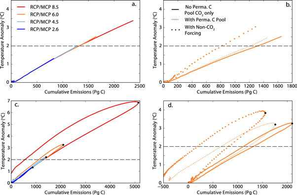
Figure 2. Temperature change versus cumulative emissions curves for: (a) the model configuration with the permafrost carbon module turned off, and forced only with changes in atmospheric CO2 for each RCP to 2100; (b) RCP 6.0 to 2100 for each of the three model configurations. (c) MCP scenarios under the same configuration as (a). (d) MCP 6.0 for each of the three model configurations. Solid line is for simulations with only CO2 forcing and with no permafrost carbon pool, the thin dotted line is for simulations with the permafrost carbon pool, and thick dotted line is for simulations with all RCP forcings. The black dashed line is the 2.0°C temperature change threshold, black dots indicate the transition point between RCP and MCP scenarios. Cumulative emissions are counted from year 1850.
Download figure:
Standard image High-resolution image
Figure 3. Evolution of temperature (a) and cumulative emissions (b) for RCP 6.0 under the model configuration with permafrost carbon but forced only with CO2 and the configuration forced with all standard RCP forcings. The simulation with all forcings is warmer and has lower diagnosed cumulative emissions at all times. Therefore non-CO2 forcing decreases the carbon budget in two ways by both (1) making the simulation warmer and (2) increasing the airborne fraction of emitted carbon. The back and red dots represent the points in time where the 2 °C target is breached for the model configuration with permafrost carbon and with non-CO2 forcing respectively. The blue cross illustrates the reduction in the carbon budget due to carbon cycle feedbacks. The black vertical line in panel (b) represents the change in the 2 °C carbon budget caused by including non-CO2 forcings.
Download figure:
Standard image High-resolution imageThe lower panels of figure 2 show the cumulative emissions versus temperature curves for the MCP simulations. The figures show that for scenarios that stay below 2000 Pg C of cumulative emissions, cooling is close to proportional to cumulative negative emissions except near the transition between positive and negative emissions. Adding the other contributing factors to climate change widens the offset between the positive and negative trajectories (figure 2 (d)).
3.2. Sensitivity of the carbon budget
Carbon budgets for 2.0 °C, 2.5 °C, and 3.0 °C temperature change thresholds for each RCP and each model configuration are shown table 1, and for each model configuration under RCP 6.0 in figure 4. Moving along the chain of model configurations reduces the carbon budgets for each for each temperature threshold. Turning on the permafrost carbon pool module reduced the carbon budget under RCP 6.0 by 105 Pg C for the 2.0 °C target, 160 Pg C for the 2.5 °C target, and 260 Pg C for the 3.0 °C target. Forcing the model with non-CO2 forcings further reduces the carbon budget under RCP 6.0 by 420 Pg C for the 2.0 K target, 440 Pg C for the 2.5 °C target, and 435 Pg C for the 3.0 °C target. The reduction in carbon budget for each model configuration, temperature target and RCP are given in table 1.

Figure 4. (a) Carbon budgets for 2.0 °C, 2.5 °C and 3.0 °C temperature change targets for the three model configurations. (b) Overshoot net carbon budgets for restoration of 2.0 °C, 2.5 °C and 3.0 °C targets for the three model configurations. Note that the overshoot net carbon budgets are smaller that the conventional carbon budgets, this implies that more CO2 must be removed from the atmosphere to return to a given temperature change than was emitted in the overshoot. Values are given for simulations following the RCP 6.0 and MCP 6.0 scenario.
Download figure:
Standard image High-resolution imageTable 1. Carbon budgets for 2.0 °C, 2.5 °C and 3.0 °C of warming under three of the RCPs. There is no model configuration where RCP 2.6 breaches the 2.0 °C warming threshold, therefore this scenario is not shown. All values are in Pg of carbon (Pg C). Change in carbon budget between model configurations under the same RCP are shown in parenthesis.
| No perma. C pool | With perma. C pool | With non-CO2 | |
|---|---|---|---|
| only CO2 | forcings | ||
| forcing | |||
| Carbon budget 2.0 °C | |||
| RCP 4.5 | 1270 | 1120 (–150) | 805 (–315) |
| RCP 6.0 | 1320 | 1215 (–105) | 810 (–405) |
| RCP 8.5 | 1340 | 1255 (–85) | 770 (–485) |
| Carbon budget 2.5 °C | |||
| RCP 4.5 | — | — | 945 |
| RCP 6.0 | 1645 | 1480 (–160) | 1055 (–430) |
| RCP 8.5 | 1700 | 1575 (–125) | 970 (–605) |
| Carbon budget 3.0 °C | |||
| RCP 4.5 | — | — | — |
| RCP 6.0 | 1970 | 1710 (–260) | 1265 (–445) |
| RCP 8.5 | 2080 | 1905 (–175) | 1190 (–715) |
If the change in temperature were exactly proportional to cumulative CO2 emissions, then under CO2 only forcing the carbon budget would be identical following each RCP path. One can see from table 1 that this is not precisely the case, and that there are small variations in the carbon budget following the different RCP CO2 pathways. From figures 2 (a) and (c). one can see that the RCP 4.5 cumulative emissions versus temperature curve is trending above the curves for RCPs 6.0 and 8.5 near the 2.0 °C threshold of warming. This reflects a small dependency of the TCRE on the rate of CO2 emissions, whereby higher annual emissions are associated with more unrealized warming in this model [35, 36]. Consequently, the TCRE for RCP 4.5 in particular, increases slightly towards the end of the simulation as emissions decrease and CO2 concentrations stabilize. This in turn has the effect of decreasing the carbon budget at the point that 2.0 °C is reached in this simulation relative to RCP 6.0 and RCP 8.5.
Turning on the permafrost carbon module reduces the carbon budget by different magnitudes depending on the RCP followed. This effect is likely related to the time-lag involved in the permafrost carbon feedback whereby the response to warming is delayed by the time taken for soils to thaw and for thawed soil carbon to decay (e.g. [15]). The slower the rate of warming the longer the permafrost carbon has been exposed to climate warming at the time the temperature change threshold is reached (e.g. [15]). This alteration of the proportionality between cumulative emissions and temperature change is consistent with the understanding of TCRE as an ocean-atmosphere generated phenomenon that becomes more dependent on the rate of CO2 emissions when strong terrestrial carbon cycle feedbacks are present [11]. Notably the UVic ESCM has a permafrost carbon feedback on the high end of the inter-model range as shown in the recent review paper of [19].
The inclusion of non-CO2 forcings reduces the carbon budget by over 400 Pg C consistently for each temperature target following RCP 6.0, but with large variation depending on the RCP followed owing to different scenarios of non-CO2 emissions. In addition to reducing the carbon budget by warming the climate directly, adding non-CO2 forcings further reduces the carbon budget by enhancing positive carbon cycle feedbacks. The contribution from these feedbacks can be quantified by examining the diagnosed cumulative CO2 emissions for a configuration forced only by changes in atmospheric CO2 at the point in time where the configuration with all RCP forcings reaches a chosen temperature target. For example under RCP 6.0 with all forcing the 2.0 °C threshold is breached in 2054 CE with a carbon budget of 810 Pg C. Forced only with CO2 cumulative emissions are 900 Pg C in 2054 CE under RCP 6.0. Therefore by turning on the non-CO2 forcings the cumulative emissions have been reduced by 90 Pg C, accounting for 22% of the reduction in the carbon budget from turning on non-CO2 forcings (see figure 3 for illustration). Table 2 shows the fraction of the reduction in the carbon budgets attributable to the enhancement of carbon cycle feedbacks from turning on non-CO2 forcings for each RCP and temperature target. This attributable fraction varies between 22% and 42% depending on the scenario and temperature target. Figure 5 shows that adding non-CO2 forcings affects carbon cycle feedbacks by reducing the uptake of carbon by the ocean and enhancing the rate of soil respiration of carbon.

Figure 5. Changes in carbon pool sizes for each RCP/MCP that breaches the 2 °C target between: the pre-industrial state and reaching the 2.0 °C temperature target (left column); the pre-industrial state and the point in time when 2.0 °C of warming is restored under each MCP (right column).
Download figure:
Standard image High-resolution image
Table 2. Fraction of the reduction in the carbon budget from including non-CO2 forcings attributable to enhancement positive carbon cycle feedbacks. Values are given for 2.0 °C, 2.5 °C and 3.0 °C temperature change thresholds.
2.0  |
2.5  |
3.0  |
|
|---|---|---|---|
| RCP 4.5 | 33 % | — | — |
| RCP 6.0 | 22 % | 28 % | 35 % |
| RCP 8.5 | 30 % | 38 % | 42 % |
Recent studies have demonstrated that given limited resources and a choice between mitigation of CO2 emissions and mitigation of short-lived forcing agents, it is always optimal to mitigate CO2 emissions [12, 37, 38]. This conclusion follows from studies showing that warming from CO2 is expected to last many thousands of years (e.g. [39]), whilst the warming from short-lived forcing agents dissipates more quickly after emissions of these agents cease. Not explicitly quantified by such analysis is that non-CO2 forcings also alter the efficiency of carbon cycle feedbacks, which here have been shown to account for 22%–42% of the reduction in carbon budget from non-CO2 forcings following the non-CO2 forcing trajectories of the RCP scenarios. Evaluating the effect of this interaction term on optimal mitigation strategy is an opportunity for future research.
3.3. Overshoot net carbon budgets
Overshoot net carbon budgets for each MCP, for temperature targets of 2.0 °C, 2.5 °C and 3.0 °C, and for the three model configurations are shown in table 3. Figure 4 displays the overshoot net carbon budgets following MCP 6.0 for the three temperature targets, and the three model configurations. In general the overshoot net carbon budgets are smaller than the positive carbon budgets, with the magnitude of the difference varying strongly with scenario and temperature target (tables 1 and 3). The difference grows larger for lower temperature targets and higher scenarios. Unlike the positive carbon budgets which are all within 200 Pg C for each scenario for a given model configuration, consistent with the concept of TCRE, the overshoot budgets are highly contingent on scenario followed. The hysteresis curves shown in figure 2(c) suggest that the path dependence of the overshoot carbon budgets is a consequence of the nonlinear relationship between carbon removal and temperature change during the transition between positive and negative emissions. Also contributing to the path dependence is the difference in the slopes of the upward and downward parts of the trajectory, where the curves are near-linear. Zickfeld et al attributes this difference in slope to inertia in ocean heat and carbon uptake [40]. The difference between positive and overshoot carbon budgets is shown in figures 2(c) and (d) by comparing the cumulative emissions at the point where the upward and downward limbs of the hysteresis curves cross the 2 °C line.
Table 3. Overshoot net carbon budgets for restoration of 2.0 °C, 2.5 °C and 3.0 °C targets following overshoot of the target. Values are giving for all MCPs that breach the target and for the three model configurations. All values are in Pg of carbon (Pg C).
| No perma. C pool | With perma. C pool | With non-CO2 | |
|---|---|---|---|
| only CO2 forcing | forcings | ||
| Anthropogenic carbon | |||
| at restoration of 2.0 °C | |||
| MCP 4.5 | 1220 | 915 | 380 |
| MCP 6.0 | 1110 | 660 | 185 |
| MCP 8.5 | 555 | −195 | –740 |
| Anthropogenic carbon | |||
| at restoration of 2.5 °C | |||
| MCP 4.5 | — | — | 680 |
| MCP 6.0 | 1415 | 975 | 430 |
| MCP 8.5 | 855 | 105 | –550 |
| Anthropogenic carbon | |||
| at restoration of 3.0 °C | |||
| MCP 4.5 | — | — | — |
| MCP 6.0 | 1780 | 1355 | 690 |
| MCP 8.5 | 1150 | 400 | –310 |
Figure 5 shows the carbon pool anomalies when the 2 °C target is breached and restored for each model configuration and for each MCP that breaches that target. All of the model configurations and scenarios show that more carbon is held in the oceans than the atmosphere when change in global temperature is returned to 2 °C. This is the opposite of what is shown at the time when the 2 °C target is breached. That is, the atmospheric concentration of CO2 is lower when one returns to the 2 °C target than the concentration was when the target was breached. This is consistent with ocean thermal inertia resisting change in climate (e.g. [31, 39]). This result also implies that the ocean's ability to assimilate CO2 counteracts the thermal inertia effect. For example under MCP 8.5 atmospheric CO2 concentration has nearly returned to its pre-industrial concentration when 2 °C of warming is restored (290 ppm), while the ocean maintains over 500 Pg C in excess carbon in the model configurations with only CO2 forcing, and over 200 Pg C in the model configuration with all standard MCP forcings.
The inclusion of the permafrost carbon module alters the carbon balance, with carbon budgets needing to accommodate the release of carbon from permafrost soils in both the positive emission and carbon removal phases of the MCPs. This can be seen in figure 5. This has a dramatic effect in the case of MCP 8.5 where the overshoot carbon budget is negative for all of the temperature targets in the model configuration with non-CO2 forcings and for the 2 °C target under the model configuration with only CO2 forcing.
Our simulations suggest that if the carbon budget for a given climate target is exceeded, more carbon must be removed from the atmosphere than the magnitude of the overshoot, if a return to the target is desired. To extend the financial analogy that carbon budgets are conceptualized from [5] if we exceed the carbon budget and go into debt we must pay back the debt with interest.
3.4. Caveats
The results presented here are from only a single intermediate complexity Earth system model and therefore should be interpreted with appropriate caution. Similar experiments with different ESMs would be needed to confirm our results. As the simulations have been performed only with the standard model parameter values we are unable to establish uncertainty bounds on these results. However, we suggest that the general features of the results captured here are of considerable interest in addition to the carbon budget values calculated by this particular model.
The version of the UVic ESCM used here does not realistically simulate the release of carbon from the land surface due to anthropogenic land use change. A better representation of these effects would partition the carbon budget between a fossil fuel budget and land use change emission budget and likely also alter the behavior of the terrestrial carbon sink.
4. Conclusions
Carbon budgets relate the primary cause of anthropogenic climate warming (cumulative CO2 emissions) to a chosen 'safe' threshold of warming (e.g. [5]). To build from the theoretical basis of carbon budgets (the proportionality between climate warming and cumulative CO2 emissions) to a real-world application of such a carbon budget requires taking into account the other contributing factors to anthropogenic climate change. In addition, one must account for the permafrost carbon pool which has yet to be included in most ESMs. Here we have examined the sensitivity of carbon budgets to these factors by sequentially turning on the permafrost carbon pool, and non-CO2 forcings to construct three configurations of the UVic ESCM. The largest reduction in the carbon budget is created by the addition of non-CO2 forcings, which reduced the budget by between 315 Pg C to 485 Pg C for the 2.0 K temperature change target, depending of the RCP trajectory followed. 22% of this reduction in the carbon budget is attributable to enhanced carbon cycle feedbacks induced by non-CO2 forcings. The permafrost carbon pool has a smaller effect reducing the budget for the 2.0 °C target by 106 Pg C when following RCP 6.0.
This experimental framework was also used to investigate the concept of an overshoot net carbon budget associated with reducing global temperatures back to a designated 'safe' temperature change target following an overshoot of such a target. The overshoot net carbon budgets are in general found to be smaller than the corresponding conventional carbon budget. The magnitude of this difference is larger given larger and longer overshoots of the carbon budget and is highly contingent on the emissions path followed. Under the most extreme scenario considered (the model configuration with non-CO2 forings under MCP 8.5) returning to 2 °C of warming requires a return to a late 19th century CO2 concentration (290 ppm) and removal of 740 Pg C more CO2 than has originally been emitted to the atmosphere. Overall carbon budgets persist as a robust and simple conceptual framework to relate the principle cause of climate change to the impacts of climate change.
Acknowledgments
K Zickfeld and H D Matthews acknowledge support from the National Science and Engineering Research Council of Canada (NSERC) Discovery Grant Program. We thank two anonymous reviewers for their constructive comments.