


Abstract
Edge localized modes (ELMs) are magnetohydrodynamic (MHD) instabilities that cause fast periodic relaxations of the strong edge pressure gradient in tokamak fusion plasmas. A novel diagnostic method allows the extraction of toroidal mode numbers, rotation velocities and spatial information during the ELM cycle including the crash. While mode number branches  –6 and
  –10 are dominant just before the ELM crash, during the ELM crash
  –5 are observed in typical discharges with type-I ELMs in the tokamak experiment. These findings are compared to results from nonlinear MHD simulations. Although
  is linearly dominant, nonlinear coupling in which
  is particularly important leads to the dominance of
  –5 during the ELM crash, in excellent agreement with experimental observations. The simultaneous occurrence of these modes over a wide radial region leads to high stochasticity and thus increased transport.
Export citation and abstract BibTeX RIS
1. Introduction
Nonlinear coupling induced fast relaxation events are not only important for magnetically confined plasmas [1], but also for astrophysical plasmas [2–4] and even in daily life mechanical systems [5, 6].
Here we investigate edge localized modes (ELMs), which are periodically appearing magnetohydrodynamic (MHD) instabilities that cause fast relaxations of the strong edge pressure gradient in highly confined tokamak fusion plasmas [7–9]. They induce intense heat and particle losses and thereby create high peak heat fluxes on the divertor tiles. This can be a major concern for future fusion devices like ITER [10, 11].
The onset criteria of ELMs is classically described by the linear peeling-ballooning boundary [12–14]. Nevertheless, linear models can only determine whether a certain mode can potentially grow. The development and the transport characteristics of modes are only accessible via nonlinear calculations, as suggested for instance by Snyder et al [15]. Nonlinear models also open up the window to purely nonlinear phenomena like saturated modes, cyclic behavior or coupling of different modes [16, 17]. Nonlinear mode coupling could also be responsible for the fast increase of growth rates at the ELM onset [18–20].
One essential parameter in order to check the validity of ELM models is the spatial structure of the mode characterized by the toroidal mode numbers n. Therefore several authors have made efforts to determine structures appearing during or close to the ELM onset with different diagnostics and methods on various machines.
Among these methods are imaging techniques from fast cameras or from 2D electron cyclotron emission [21–25]. Those methods mainly rely on estimating the distance between several maxima of the modes. This is correct as long as there is only one dominant structure present. For other cases, these methods might not give access to the full mode spectrum since they neglect the interference of the different Fourier components [26]. This is maybe also a reason why in most of these cases quite high mode numbers in the range of  –30 are observed during the ELM crash.
The most commonly used diagnostic for calculating the structure of modes close to the ELM crash are magnetic pick-up coils measuring either radial or poloidal magnetic field changes. These pick-up coils are arranged in arrays spread along the toroidal angle. From these signals exact mode structures n are determined by a proper Fourier decomposition. Various types of modes are seen on different machines in the edge region that are thought to be important for the whole ELM cycle. They appear in a wide range of frequencies below 500 kHz.
Some of them are usually stationary for up to several milliseconds in a high frequency range of 100–500 kHz with several frequency bands of mode numbers around  and separated by
  [27–30]. They propagate in the lab frame in electron diamagnetic direction. Their phase velocity is controversially discussed in the listed references. They are also regarded as being responsible for clamping the gradient in between ELM crashes [31, 32], but not being directly connected to the ELM crash. The clamping of the gradient fits to the EPED model [14], which states that the transport induced by kinetic ballooning modes (KBM) is an important ingredient for the pedestal height and width in the ELM cycle. Nevertheless, only some of the important mode properties like stability characteristics or structure size were found to fit to KBMs. Others like rotation velocity or symmetry have large errors or even contradict KBMs.
Other parts of the modes investigated in the ELM cycle appear in magnetics in a lower frequency range of 0–150 kHz. They also appear with several frequency bands and usually with lower mode numbers  . Their rotation direction in the lab frame seems to differ between machines. As they tend to appear and grow before the ELM crash, they are often called precursors. In which way they are linked to the crash is not yet clear [28–30, 33, 34].
The modes that appear during the crash itself are with magnetics only in very rare cases reliably studied [35, 36], but usually very low mode numbers of  –4 are found dominantly during the crash.
In this paper, we report for the first time on measurements by magnetic pick-up coils on the ASDEX Upgrade tokamak [37] which were able to decompose the slowly propagating, short-lived toroidal sub-structure of the ELM cycle including the ELM crash and the ELM precursor modes. This is done via ELM synchronization of temporal Fourier analysis, which allows to determine not only the structure but also rotation velocities of the ELM. The experimental findings in terms of mode numbers, velocities, growth rates and kinetic profiles during the crash are then compared to results from the nonlinear MHD code JOREK [1].
2. Experimental investigations
The ASDEX Upgrade discharge #33616 was considered to determine the structure of the modes appearing before and during the ELM crash. In this discharge, a long constant phase with a plasma current of 800 kA, magnetic field of 2.5 T, total heating power of 4 MW, edge safety factor  and with a low ELM frequency of around
  Hz was obtained. ELM induced losses of thermal energy and particles were of about 6
 and 8
and 8 respectively, during which the maximum pedestal pressure gradient drops by a factor of three. Figure 1 shows a magnetic spectrum from the low field side (LFS) midplane, synchronized to the onset at
  ms of 52 similar ELMs from this constant phase. The onset and end of the ELMs are defined from an amplitude threshold in the magnetics. This definition is similar to divertor signals like
  or shunt current measurements, but reduces smearing of synchronized magnetic signals to ⩽0.1 ms. The spectrum is measured with a radial magnetic field coil. Several milliseconds before the crash, saturated modes with frequencies around 200–250 kHz are visible. These modes appear together with the clamping of the pedestal pressure gradient [32]. On the other hand medium frequency fluctuations at 10–125 kHz are visible and their amplitude increase about 2 ms before the crash, which is why they are called precursors in the following.

Figure 1. Spectrum taken from LFS midplane coil synchronized to the ELM onset at  ms of 52 ELMs. 10–125 kHz fluctuations increase about 2 ms before the crash, which itself is then dominated by low frequencies
 kHz.
kHz.
Download figure:
Standard image High-resolution imageDuring the ELM crash,  –2 ms, the spectrum is broad in frequency, but the low frequencies (
 20 kHz) are the most dominant ones. Growth rates of the magnetic amplitude
  at the onset are of the order of
 . This growth rate was estimated from a sliding average with 150
 s length and 15
 s separation. Such filtering is necessary in order to reduce the effect of noise in the magnetics.
In order to obtain the toroidal structure of the different modes forming the different frequency bands, a toroidal array of magnetic pick-up coils is installed on ASDEX Upgrade. The mode numbers can be calculated from the relative phases of the magnetic fluctuations between these toroidally separated coils. A detailed description of the method is given in [29]. Figure 2 shows two ELM synchronized mode number spectra. The negative sign of mode numbers in the spectrum by convention indicates a rotation in the direction of the electron diamagnetic drift and is omitted in the text for readability. These plots are obtained by determining mode numbers that appear in a window of 2.2 ms duration. The center of these windows are 1.2 ms before and 1.0 ms after the ELM onsets respectively for a) and b). The 2.2 ms are needed in order to get a good frequency resolution. In that sense it is an average over the whole crash event and cannot resolve the detailed evolution during the crash. Evaluated time windows are also marked with white dashed lines in figure 1. The resulting mode numbers of all these windows around the 52 ELM onsets in the here investigated time trace are then binned together. Below  kHz the spectrum is influenced by an
  ,
,  core mode. As the core mode is not expected to have a strong impact on the edge, the mode number spectrum in figure 2(a) is blue shaded below the grey dashed line at
  kHz to guide the eye towards the ELM relevant medium to high frequency edge fluctuations. Before the ELM onset the spectrum is dominated by the high frequency fluctuations with
  . Then, close to the ELM onset, precursor fluctuations with
  with frequencies 35–125 kHz increase in intensity.

Figure 2. Frequency resolved mode number spectra of a time window (a) shortly before and (b) during the ELM crash. The low n sub-structure of the pre-ELM components appears with strongly reduced  but similar dominant
  also during the crash.
Download figure:
Standard image High-resolution imageThe total velocity, i.e. toroidal, poloidal and phase velocity, determines together with n the frequency of the modes. The n-components of similar  rotate with the same velocity. Due to the strong shear of the edge rotation it is highly probable that the structures
  at frequencies of around 200, 225 and 240 kHz (green arrow) before the onset are at the same position in the plasma. The same holds for the
  components with frequencies of 80, 100, 120 kHz (red arrow). The
  component is the slowest one with
  kHz (white arrow). Compositions of several n-components at the same radial position are called mode branches in the following. The n-components in such a branch are prone to coupling as they have same velocity and position.
The uncertainty of 1–2 kHz in  reflects a width below 5 mm of the mode branches in the strongly sheared edge rotation. A precise determination of the radial position is not possible from the rotation as the errors in the measurement of the radial electric field are too big and the phase velocities of the modes are unknown. Nevertheless, measurements of the poloidal mode numbers show for the
  component of the slower branch
  , whereas
  –60 for the
  component of the faster branch. This suggests that slower mode branches of the precursor modes have higher
  and are therefore located further outside close to the separatrix, whereas mode branches with high
  have lower
  and are placed further inwards close to the
  minimum which is usually around
  for this type of discharges.
During the crash, figure 2(b), the dominant mode numbers are  , which is very similar to the preexisting
  structure. This low n structure during the crash is a general feature of many ASDEX Upgrade discharges, which only varies very slightly with usual parameters like
  or β. It appears with
  kHz (note the different scaling of the frequency axis). This reduction of velocity compared to the precursor is a result of the
  reduction at the ELM onset from typically 40 to 10 kV
  and thereby a relative increase of the toroidal velocity component which is in the ion drift direction [38, 39]. Another ingredient for the velocity reduction might be an additional outwards propagation into the region of reduced absolute
  and a possible coupling due to increased mode amplitude to external error fields leading to a braking of the rotation.
3. Nonlinear simulation of the ELM crash
The novel experimental techniques described in the preceding paragraphs form an excellent basis for comparing simulations and experiments. With this in mind, an ELM simulation is carried out with the nonlinear MHD code JOREK [1] based on a CLISTE [40] pre-ELM equilibrium reconstruction of discharge #33616 at  s which is peeling-ballooning unstable. The reconstructed equilibrium is based on kinetic profiles just before the ELM crash averaged over several ELM cycles from Thomson scattering, Li-beam and ECE diagnostics [41–43]. The computational domain covers main plasma, scrape-off layer (SOL) and private flux region including geometrically simplified divertor targets where Bohm boundary conditions apply (refer to [44, 45] for the model). Diamagnetic and neoclassical flows are included, background parallel flows inside the plasma are not considered for simplicity since they do not affect the ELM crash strongly due to the large parallel wave length of the ELM structures. Plasma resistivity is significantly more realistic than in previous ELM simulations for ASDEX Upgrade [19, 46] but still a factor of eight larger than the experimental value for computational reasons. Note that these earlier simulations also did not account for diamagnetic drift effects such that much higher mode numbers had been obtained due to this missing two-fluid stabilization term acting on high mode numbers. Scans confirm that time step, resolution, hyper-resistivity and viscosity do not influence results. The parallel heat diffusion coefficient is chosen about two orders of magnitude smaller than the Spitzer-Härm values [47] to account for the so-called heat flux limit [48, 49]. Additional details regarding the simulation setup can be found in appenix. The simulation includes toroidal mode numbers
  –8. Linear analysis and single simulations with mode numbers up to 16 showed that
  modes are strongly subdominant and need not be considered in this case. Note that this is in contrast to the
  modes observed in the inter-ELM phase experimentally (however not during the ELM crash itself). The absence of these modes in simulations can have two different reasons: either the initial conditions do not reflect accurately enough the experimental state, or these modes cannot be described in the MHD picture.
Time traces of the most important quantities from the simulation around the ELM crash are shown in figure 3. From a small initial perturbation (only visible on logarithmic scale, see left part of figure 3), the peeling-ballooning instability starts to grow exponentially from time  ms. All times for the simulation are given relative to the ELM onset time
  defined by the start of the rise of the outer divertor heat flux in the simulation due to the crash. This makes the timing comparable to the one in the experiment.
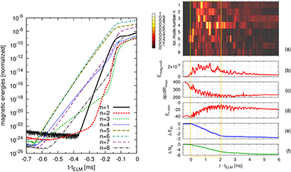
Figure 3. Left: time traces from the simulation are shown of magnetic energies on a logarithmic time scale for the onset of the ELM crash. Right: time traces from the simulation are shown of (a) magnetic energy (a.u.) for each toroidal mode number  –8, (b) sum of the magnetic energies for
  (a.u.), (c) maximum pressure gradient in the midplane (kN
  ), (d) minimum of Er in the midplane (kV
  ), (e) losses of thermal energy (%), and (f) particle losses (%). The vertical lines mark the beginning and end of the ELM crash.
Download figure:
Standard image High-resolution imageThe  and 5 components are linearly dominant with a growth rate of about
 . From
  ms, nonlinear drive of sub-dominant mode numbers [19] (first
  by a coupling of
  ) can be observed, and at about
  ms nonlinear saturation starts to set in.
During the ELM crash itself (right part of figure 3), from about  ms to
ms to  ms, thermal energy and particle losses are observed across the separatrix. About 2.5
 of thermal energy and 7
 of particles are lost (figures 3(e) and (f)). The divertor heat flux starts to rise at
  ms for the outer and at
  ms for the inner target. During the ELM crash,
  –5 modes are dominant while
  modes remain strongly sub-dominant (figure 3(a)). The spatial structure of the instability simultaneously involves several rational surfaces rotating with different velocities corresponding to the different branches observed in the experiment. Additional simulations were carried out to identify key ingredients for obtaining the experimental mode spectrum. Restricting the mode numbers included in the simulation to
  or
or  instead of the full spectrum (
 –8) leads to an almost pure
  during the ELM crash and when excluding diamagnetic flows,
  modes dominate. This highlights that the spatial structure of the ELM is reproduced in the simulations only when taking into account the diamagnetic drift term and accounting for nonlinear mode coupling involving
  . In particular, the toroidal mode structure differs significantly from the linear spectrum.
The maximum pressure gradient in the outer midplane drops approximately by a factor of two during the crash (figure 3(c)) and the radial electric field (Er) well is reduced from about  to
to  kV
kV  (figure 3(d)) leading to a much lower
  rotation. After the crash, magnetic fluctuations drop significantly and energy and particle losses cease. Pressure gradient and Er well slowly start to recover. Fluctuating inter-ELM modes dominated by
  persist until about
  ms. Then a slowly evolving
  structure becomes dominant for more than
  ms. Due to the ELM crash,
  and
and  islands arise with a width of
  cm, which decay away slowly such that they would clearly 'survive' until the next ELM crash. The experimentally observed seeding of neoclassical tearing modes by ELMs (e.g. [50, 51]) could, thus, be a cumulative result of several ELM crashes.
In the region  , field lines become stochastic during the ELM and closed flux surfaces only recover slowly after the crash8. Stochastization can be observed inwards up to
  in certain phases (figure 4 for simulation time
  ms). Stochastic fields are important for the ELM energy losses and thus for the ELM dynamics. For the formation of the stochastic layer, the excitation of several toroidal mode numbers by nonlinear mode coupling is important since it modifies the edge magnetic topology and thus the connection from bulk plasma to the divertor.
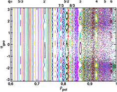
Figure 4. A Poincare plot is shown in radial and poloidal coordinates to illustrate the magnetic topology during the ELM crash obtained in the JOREK simulation ( ms).
ms).  corresponds to the outer and
  to the inner midplane, the X-point is located at
  . Safety factor values corresponding to some of the island chains are given at the top.
Download figure:
Standard image High-resolution image4. Conclusion and discussion
A novel experimental tool was developed, which allows extraction of key information about ELM crash and inter-ELM activity.
Experimental observations and the nonlinear ELM simulation show excellent agreement regarding key features such as the ELM duration of about  ms, growth rates in the order of
 and the dominant toroidal mode numbers
  –5 during the crash. Note that the growth rates in the simulations are determined by equilibrium reconstruction, physics parameters, and background flows such that a really self-consistent comparison will only be possible with full ELM cycle simulations at fully realistic parameters. In both cases mode numbers larger than 6 are clearly sub-dominant, which is also in agreement with previous experimental investigations [35, 36]. Nonlinear mode coupling involving the
  component as well as diamagnetic drift are key ingredients for obtaining this spectrum in simulations. In the simulation, thermal energy ELM losses are smaller than in the experiment by a factor of about two (2.5% versus
  ) and particle losses are almost identical (
 versus
  ). Accounting for time-varying background turbulence levels during the ELM cycle and treating the heat flux limit of parallel transport more accurately might allow to resolve this discrepancy. Edge stochastization in the modeling is responsible for the fast temperature collapse in the plasma edge due to the fast parallel heat transport, highlighting the role of reconnection for this process during the ELM crash [52].
In the experimental analysis (figure 2(b)), a relatively broad frequency spectrum is observed during the ELM crash which can be explained by several effects observed in the simulation: changing rotation during the crash, a radial mode structure spreading over several rational surfaces with different local rotation velocities, and fluctuating amplitudes within the analysis window. Furthermore, the important  component visible in modeling might not be accessible to the temporal Fourier analysis due to its long wavelength and short life span which do not allow to measure a full oscillation period. A one-to-one comparison via virtual diagnostics is planned for the near future using the free-boundary extension JOREK-STARWALL [53].
Before the crash, a precursor mode with a similar mode structure as the crash is observed experimentally. Unfortunately, this phase can also not be compared to the simulation yet which was started from an unstable equilibrium already. Simulations started from a stable state, where the plasma is crossing the stability boundary due to the build-up of pedestal profiles are planned for the near future. Those simulations might also show saturated modes when the equilibrium is only barely unstable and a sudden crash when the ideal ballooning stability boundary is reached. Magnetic fluctuations after the ELM crash are roughly a factor of five smaller than during the ELM crash in experiment as well as in modeling. This magnetic activity is correlated with fluctuations of density and temperature in the pedestal region which do not cause strong losses and are also observed experimentally in ECE-Imaging measurements in the inter-ELM phase [54].
Significant progress in the experimental analysis of ELM crashes has been obtained and strong evidence was shown that JOREK nonlinear simulations reproduce key aspects of ELM crashes. Future experiments will investigate the effect of parameter variations on ELM precursor and crash. Future simulations will aim at realistically obtaining the whole dynamics of the ELM cycle. Similar comparisons are also planned for ELM suppression scenarios and natural ELM free states.
Acknowledgments
This work has been carried out within the framework of the EUROfusion Consortium and has received funding from the Euratom research and training programme 2014–2018 under grant agreement No 633053. The views and opinions expressed herein do not necessarily reflect those of the European Commission.
Appendix. Details on the simulation setup
The simulations are based on a CLISTE equilibrium reconstruction using pre-ELM profile measurements (the corresponding ASDEX Upgrade shot file is found at micdu:eqb:33616:1:7.2s). The safety factor and pressure profiles are shown in figure A1 along with the finite element grid used for the simulations (about 14 000 elements in the poloidal plane). The resistivity is given by  where T0 denotes the initial temperature in the center of the plasma, and
  in normalized units corresponding to about
  in SI units. The viscosity profile is set up with the same temperature dependency and an initial center value of
  in normalized units corresponding to about
  . Neoclassical effects are considered in the form of a neoclassical tensor similar as described in [44], using constant coefficients: neoclassical friction is
  in normalized units, corresponding to about 17.7
  , and neoclassical heat conductivity is
  . Hyperresistivity and hyperviscosity are spatially constant and set up in a way that in the region of the instability
  and
and  ensuring that they do not influence simulation results. Heat and particle source profiles are very simplified, and the perpendicular heat and particle diffusion coefficients are set up in a way that on the time scale of the ELM crash, profiles do not change significantly in an axisymmetric simulation without instability. This in particular means they are strongly reduced in the pedestal region to model the edge transport barrier. A more careful setup of sources and diffusivities in line with experimental measurements is required in future cases to simulate full ELM cycles. The JOREK input files are available upon request. The JOREK version used to perform the simulation corresponds to version 8206ec4bd37325e2dad0cb44356ceae31b942d2a of the develop branch in the central git repository as of November 30th 2016.

Figure A1. Left: the flux surface aligned X-point grid and the separatrix are shown as used for the simulation setup. Right: profiles of safety factor and pressure as used for the simulation are plotted.
Download figure:
Standard image High-resolution imageFootnotes
- 8
 where and Ψ the poloidal magnetic flux.

