
Abstract
Objective. Currently, few non-invasive measures exist for directly measuring spinal sensorimotor networks. Electrospinography (ESG) is one non-invasive method but is primarily used to measure evoked responses or for monitoring the spinal cord during surgery. Our objectives were to evaluate the feasibility of ESG to measure spinal sensorimotor networks by determining spatiotemporal and functional connectivity changes during single-joint movements at the spinal and cortical levels. Approach. We synchronously recorded electroencephalography (EEG), electromyography, and ESG in ten neurologically intact adults while performing one of three lower-limb tasks (no movement, plantar-flexion and knee flexion) in the prone position. A multi-pronged approach was applied for removing artifacts using  filtering, artifact subspace reconstruction and independent component (IC) analysis. Next, data were segmented by task and ICs of EEG were clustered across participants. Within-participant analysis of ICs and ESG data was conducted, and ESG was characterized in the time and frequency domains. Generalized partial directed coherence analysis was performed within ICs and between ICs and ESG data by participant and task. Results. K-means clustering resulted in five clusters of ICs at Brodmann areas (BAs) 9, BA 8, BA 39, BA 4, and BA 22. Areas associated with motor planning, working memory, visual processing, movement, and attention, respectively. Time-frequency analysis of ESG data found localized changes during movement execution when compared to no movement. Lastly, we found bi-directional changes in functional connectivity (p < 0.05, adjusted for multiple comparisons) within IC's and between IC's and ESG sensors during movement when compared to the no movement condition. Significance. To our knowledge this is the first report using high density ESG for characterizing single joint lower limb movements. Our findings provide support that ESG contains information about efferent and afferent signaling in neurologically intact adults and suggests that we can utilize ESG to directly study the spinal cord.
Export citation and abstract BibTeX RIS

Original content from this work may be used under the terms of the Creative Commons Attribution 4.0 license. Any further distribution of this work must maintain attribution to the author(s) and the title of the work, journal citation and DOI.
1. Introduction
Spinal cord injury (SCI) is a debilitating and life-long condition affecting approximately 302 000 people living in the United States alone, with an average of 18 000 new cases of SCI each year [1]. The costs associated with SCI are substantial, with lifetime cost estimates that can reach $5.8 million (USD) depending on the severity of the injury and age at injury [1]. While other areas of healthcare have improved-for example, people with HIV have seen a dramatic increase in life expectancy since the disease was first identified in the 1980s-the same cannot be said for SCI [2]. In fact, the average years of life for a person with SCI have not improved since the 1980s and remain significantly lower than that of a person without SCI [1].
One potential area for improvement is the way SCI is categorized. Currently, the severity of an SCI is ranked using the American Spinal Injury Association Impalement Scale (AIS). This scale uses a binary approach, ranking from AIS 'A', where a person has no motor or sensory function in the sacral segments, to 'E', where a person has an SCI but motor and sensory function are normal [3]. However, this fails to address the heterogeneity of injury, where each SCI is unique to itself and that even within AIS A patients, different levels of injury (thoracic T2-T10 and thoracolumbar T11-L2) had significantly different motor improvements [4].
While electroencephalography (EEG) has been used for non-invasive study of the brain and has led to different ways to predict or diagnose disease, seizure, and decoding intent, there are few non-invasive methods to study the spinal cord [5–7]. Researchers typically treat the spinal cord as a black box. One method is to apply a known physical or electrical perturbation to the body or spinal cord and relate the response to the stimulus [8, 9]. In this case, the output (e.g. movement or changes in movement) is used to infer the underlying motor network behavior. An alternative approach is modeling; for example, high-density electromyography (hdEMG) can be decomposed and related to the activity of spinal motor pools [10]. While these approaches can be very effective at characterizing the underlying circuitry of the spinal cord and the behaviors, they are limited in the amount of information provided; namely, they provide information only regarding changes in the spinal cord related to the movement being performed.
One approach to filling this gap is to use electrospinography (ESG). ESG is a well-studied technique that utilizes one or more surface electrodes placed over different areas of the spinal column and is typically used to record evoked responses from electrical stimulation to peripheral nerves and to monitor the spinal cord during surgery [11, 12]. It has been demonstrated that these responses are spinal cord in origin and, while significantly lower in amplitude, have the same characteristics as their invasively recorded counterparts [12, 13]. However, little research has been done to determine if ESG can be utilized for other applications such as decoding intent, with only a single study known to the authors that shows a proof of concept [14].
In this study, we systematically investigate the use of high-density ESG with neurologically intact participants. First, we recorded EEG, ESG, and electromyography (EMG) simultaneously during single joint movements. We demonstrate that by using an adaptive filtering algorithm, we can effectively remove cardiac artifacts from ESG. Next, we characterize the power spectral density (PSD) changes in the ESG signal during movement and compare them against sensors placed away from the ESG array. Lastly, we look at the changes in functional connectivity between cortical areas and the spinal cord during movement preparation and execution.
2. Methods
2.1. Participants
Ten neurologically intact participants (Height: 165 ± 15 cm, Weight: 72 ± 8 kg, Age: 30 ± 12 years, Sex: 4 women) were recruited to participate in this study. Written informed consent to the experimental procedures, which were approved by the University of Houston institutional review board, was obtained from each participant. This research was conducted in accordance with the principles embodied in the Declaration of Helsinki and in accordance with local statutory requirements [17]. Figure 1 provides an overview of the experiment setup ((A) and (B)) and outlines the experimental protocol (C) used in this study.
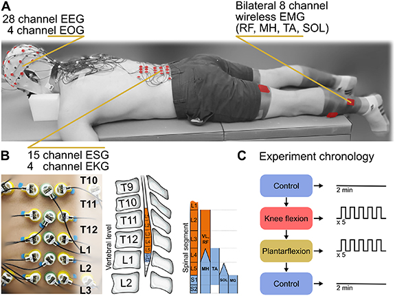
Figure 1. Experimental protocol: The experiment was performed with (A) the participant in the prone position while measurements were taken with 28-channel electroencephalography (EEG), 4-channel electrooculography (EOG), 15-channel electrospinography (ESG) with 4 channels for noise around the ESG array, and 8-channel electromyography (EMG)/ inertial measurement unit (IMU). ESG was recorded at the intervertebral spaces starting at T10/T11 and ending at L2/L3 (B) which corresponds to the approximate location of the lumbar enlargement. The participant performed one of three movement tasks (C), a no movement control condition, knee flexion of the left or right leg, and plantarflexion of the left or right foot. These tasks were repeated for 5 blocks of 5 repetitions per block for a total of 25 repetitions per movement per leg, with at least two minutes between conditions and one minute between repetitions. The control condition (no movement) was performed twice for two minutes at the start and end of the movement conditions. Spinal segment chart adapted from [15] and utilizes data from [16]. Reproduced with permission from [15]. © 2015 the American Physiological Society.
Download figure:
Standard image High-resolution image2.2. Experimental setup
EEG and ESG data were recorded with (Brain Products GmbH, Morrisville, NC) active Ag/AgCl electrodes amplified via a Brain Products BrainAmp DC amplifier (Brain Products GmbH) at a sampling frequency of 1000 Hz through BrainVision Recorder software (Brain Products GmbH).
Thirty-two channels of EEG were placed following a modified 10–20 international standard arrangement. Channels TP9, TP10, PO9, and PO10 were removed from the cap and utilized for electrooculography (EOG) to measure eye movements and eye blinks. The EOG channels were arranged so the sensors TP9 and TP10 were placed on the left and right temples, respectively, and PO9 and PO10 were positioned superior and inferior to the right eye, respectively. Ground and reference were placed on the left and right earlobes, respectively.
Nineteen channels of ESG were placed between the intervertebral spaces, starting at T10/T11 through L2/L3, found via palpation. Where three sensors were placed at each intervertebral level, with the middle sensor placed along the midline of the spinal column and the left and right sensors placed directly next to the midline sensor. Four additional sensors were placed bilaterally, approximately 5 cm from the midline, just above and below the array. These sensors were utilized to measure EMG, cardiac (EKG), and other artifacts. The electrode impedance was maintained below 25 kΩ which was verified prior to the start of and after the completion of the experiment. To prevent excessive flexion of the neck while the participant was in the prone position, a face-down foam support was used.
Trigno Avanti wireless surface EMG electrodes (Delsys Inc. USA; common-mode rejection ratio  80 dB; size: 27 mm × 37 mm × 13 mm; input impedance:
  1015 Ω/0.2 pF) were placed at eight different sites: bilaterally over the rectus femoris (RF), the medial hamstring (MH), the tibialis anterior (TA), and the lateral aspect of the soleus (SOL) muscles. EMG data were amplified by a Trigno Avanti amplifier (Delsys Inc.; gain: 909; bandwidth: 20 to 450 Hz). Each sensor contains an integrated 9-degree of freedom inertial measurement unit (IMU) (3-axis accelerometer; sampling resolution: 0.016 ± 0.001 g/bit; noise:
  0.01 g RMS; resolution: 16 bit; 3-axis gyroscope; range: ± 2000∘, and 3-axis magnetometer; range: ±4900 uT). EMG and IMU data were sampled at 1925 Hz and 148 Hz, respectively. In addition to the adhesive backing used to attach the sensor to the skin, an elastic underwrap athletic foam tape was used to hold the sensors in place to minimize movement artifacts.
2.3. Experimental procedure
Participants were asked to perform one of three tasks: (1) no movement (control), (2) plantarflexion of the left (LPF) or right (RPF) foot, and (3) knee flexion of the left (LKF) or right (RKF) leg, with all participants performing both left and right movements. Prior to the start of each task, participants were given a demonstration of the movement they were to perform, instructed to remain relaxed between repetitions, and to move only the targeted joint to the best of their ability. Movement tasks were performed in five blocks of five repetitions for a total of 25 receptions per movement. Movements were self-paced, and the participant was told to start the block 1–2 s after a verbal cue signifying the start of the block. The time between conditions was no less than 2 min, and blocks within a given condition occurred no less than 1 min apart. The control task (no movement) was performed for 2 min each time preceding and following the two movement conditions to account for possible changes in resting-state cortical and spinal activity over the course of the experiment [25].
2.4. Signal pre-processing
Signal pre-processing and statistical analysis were performed off-line utilizing custom software written in MATLAB R2022b (MathWorks, MA) and included functions from the open-access toolbox EEGLAB [19]. A flowchart outlining the signal pre-processing pipeline and analysis is shown in figure 2 and follows a previously utilized pre-processing methodology [24].
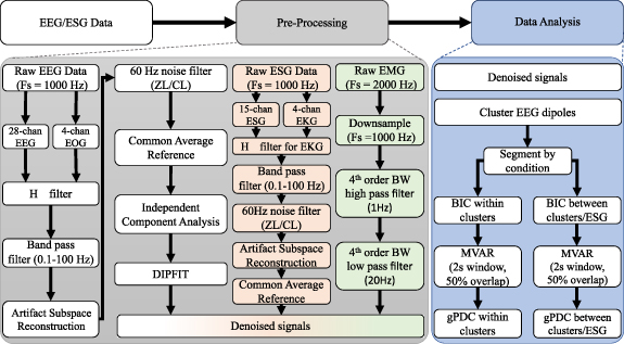
Figure 2. Electroencephalograph (EEG) and Electrospinography (ESG) data denoising and analysis: Raw EEG data were cleaned by applying an  filter which uses electrooculography (EOG) recordings [18] to identify and remove ocular artifacts, signal drifts, and other shared sources of noise. The data are then band-pass filtered (0.1–100 Hz) using a 4th order ButterWorth filter, line noise was filtered via two different complementary adaptive filters, then artifact subspace reconstruction (ASR) was done to remove other types of artifacts. The data were common average referenced, then independent component analysis (ICA) was utilized to further identify and remove any remaining artifacts. Finally, the algorithm DIPFIT was applied to determine the equivalent dipole locations for each IC [19]. Raw ESG data were cleaned by applying an
  filter with different filter weights (q = 10−7, γ = 1.2) and using recordings around the array to identify and remove cardiac artifacts and other sources of shared artifacts. Then data were band-pass filtered and line noise was filtered utilizing the same method that was applied to EEG, then ASR was performed. Lastly, the data were common average referenced. Raw EMG was downsampled to 1000 Hz, then bandpass filtered using a 4th order ButterWorth (BW) filter to determine the envelope of activation. Analysis of the cleaned data included using Bayes information criterion (BIC) [20, 21] to determine the best model order, creating a multivariate autoregressive model (MVAR) [22] and calculating the generalized partial directed coherence (gPDC) [23] within clustered EEG dipoles and between clustered dipoles and ESG sensors. The EEG data pre-processing (denoising) and analysis methodologies were adapted from [24].
Download figure:
Standard image High-resolution image2.5. EEG pre-processing
EOG data (4 channels) were used to filter the EEG signals (28 channels) via  an adaptive algorithm that removes artifacts such as eye blinks or eye movements (q = 10−9, γ = 1.15) [18]. The data were then zero-phase band-pass (0.1 Hz–100 Hz) filtered by applying a fourth-order ButterWorth filter.
Next, artifact subspace reconstruction (ASR) was performed to remove high-amplitude artifacts (e.g. muscle activity, sensor movement, wire tugs, etc). Just prior to the start of the experiment, 2 min of EEG recorded with the participant in the prone position without movement were taken as calibration data for ASR and were not utilized as the control condition during the experiment. Corrupted subspaces were reconstructed utilizing the neighboring channels and a mixing matrix that is computed by the covariance matrix via the calibration data. For this process, a sliding window of one second and a variance threshold of four standard deviations were implemented to identify and rebuild the corrupted subspaces.
Two complementary adaptive filters were applied to remove harmonics of 60 Hz power line noise (CleanLine and ZapLine Plus toolboxes for EEGLAB) [19, 26–28]. The EEG channels were then re-referenced by subtracting their common average. Next, using the standard three-shell boundary element head model included in the DIPFIT toolbox, the equivalent dipole that matched the scalp projection of each independent component (IC) was computed [19]. Each IC scalp projection, the equivalent dipole's location, and the power spectra were then visually inspected, and ICs that related to non-brain artifacts (e.g. sensor movement, muscle artifact, etc) were removed from the analysis.
2.6. K-means clustering
To establish a common group-level comparison of EEG data at the cortical source level, K-means clustering was performed. Specifically, equivalent dipoles of ICs that explained greater than 80% of the data variance were retained for dipole clustering. The number of clusters was determined by three different algorithms (Calinski–Harabasz, Silhouette, Davies–Bouldin) so that the best fit could be achieved [29–31]. This process concluded that the best fit was k = 5, 5, and 9 for Calinski–Harabasz, Silhouette, and Davies–Bouldin, respectively. Because two of the algorithms returned the same value, the ICs were clustered by applying the k-means algorithm with k = 5 centroids and dipoles were clustered using the squared euclidean distance with respect to equivalent dipole locations only, which was done to avoid circular inference [32]. If an IC with a dipole whose distance from a cluster centroid was more than three standard deviations, it was omitted from further analysis. This resulted in a total of 107 ICs being retained across participants and clusters for further analysis.
2.7. ESG pre-processing
Four channels, placed bilaterally 5 cm lateral to the midline and approximately parallel to the top and bottom of the lumbar ESG array, were utilized to filter EMG, EKG, and other sources of noise. These sensors are referred to in the text as 'EKG sensors.' The EKG sensors were utilized by the  adaptive filtering algorithm, similar to what was used prior for eye artifacts in the EEG recordings.
In this case, two values q and γ were adjusted for this application (q = 10−7, γ = 1.2). Specifically, the  adaptive weight estimation filter with time varying weights can formulated such that
where  is the estimated weight per channel at sample i + 1, ri
is a vector of reference measurements, in this case the EKG sensors, yi
is defined such that
is the estimated weight per channel at sample i + 1, ri
is a vector of reference measurements, in this case the EKG sensors, yi
is defined such that

where

and  is the noise covariance matrix which satisfies the equation

which is initialized with  where µ is a constant. gamma is the bound on the energy-to-energy gain from the disturbances to the output estimation error and defines the levels of disturbance tolerated by the
  filter.
In this formulation the weights are assumed to be time-varying with unknown variation dynamics and when γ < 1 the filter provides a guaranteed robust performance under all levels of disturbances in the system and the formulation is valid for the inequality  where
where  is the supremum of the measured disturbances and q reflects the a priori information of how rapidly the weights vary over time. Thus, by adjusting both the selected value of γ and q, we can modify the behavior of the
  filter for both applications [18].
The data were then zero-phase high pass filtered by applying a fourth order ButterWorth filter with a cut off frequency of 0.1 Hz. Then ASR was performed using a sliding window of 1 s and a variance threshold of four standard deviations. To remove harmonics of 60 Hz power line noise the approach previously outlined for EEG data cleaning was applied (CleanLine and ZapLine Plus toolboxes for EEGLAB) [19, 26–28]. Lastly, ESG channels were re-referenced by subtracting their common average.
2.8. Power spectral density
The data were segmented by condition, then by block, where each condition had five blocks consisting of five repetitions. First, PSD was calculated with a 750 ms sliding window using 99% overlap to apply Thomson's multitaper estimate in MATLAB, with 4990 frequency bins (0.1–50 Hz) and a half-bandwidth product of four for the entirety of each block [24, 33].
Next, the PSD data were further segmented by start and stop periods, where a movement that caused EMG changes larger than two standard deviations from the mean was defined as the start of the movement, and the end of the movement was defined as the point where EMG returned below this cutoff. PSD data was averaged over windows that fell completely within the movement period. To compare to the baseline, the same number of windows were taken between 5 and 20 s prior to the first movement within each block. The data were averaged across repetitions and blocks within individual participants. ESG sensors were analyzed using a bipolar configuration to reduce common noise and increase differences between ESG sensor pairs.
Next, to determine the effect noise had on the resultant data, the PSD was also calculated using the four EKG sensors at the same time points and analyzed by sensor.
2.9. Functional connectivity
Figure 2 (data analysis) provides a flowchart of the steps taken to determine generalized partial directed coherence (gPDC) from within participant clustered IC data, where IC's belonging to the participant were selected, and between participant IC's and ESG data, which was modified from a previously utilized methodology for determining functional connectivity [24]. Due to the differences in signal characteristics between the cortical sources and ESG recordings, we expected the model orders that best described the clustered data only and the model orders that best described the entire data (e.g. connectivity between clustered ICs and ESG) would be different. For that reason, two models were utilized to best represent the two pathways.
Using this method, two models were created for each participant, utilizing the ICs in the clusters belonging to that participant only and the participants' ICs and their respective ESG data, which was vertically concatenated with the IC data. Each model was computed from a model order p = 4 to 100 for each condition and each participant, then stored in a matrix where the first row is the minimum BIC value calculated between the ICs for that participant and the second row is the minimum BIC determined for the participant ICs and their respective ESG data. Therefore, each column represents the minimum BIC for that condition for the two models, and each model order matrix represents one participant.
Next, the mean of each row in the model order matrix is calculated, and a final multivariate autoregressive (MVAR) model with a two-second window and 50% overlap is constructed for each participant and condition using the determined model order [22, 34]. The MVAR model can be described by the equation
in which X(n) is a multivariate M-channel process of length n, Ak
are MxM parameter matrices that are comprised of the coefficients  that relate the ijth series at lag m and describe the interactions between time series pairs over time. The vector of model innovations E has a zero mean and a covariance matrix
  , and the model order p is the corresponding model value.
To determine information flow, gPDC was applied because to the MVAR models because it can be utilized to determine directional influences and can detect the interaction of multiple influences (M > 2) [23, 35]. The gPDC equation is given as
where  is the Fourier transform of MVAR model coefficients Ak
,
is the Fourier transform of MVAR model coefficients Ak
,  is the i jth element of
  ,
,  signifies the complex conjugate operation. The difference between gPDC and PDC is a normalization factor used to correct for cases where the innovation matrix is unbalanced which occurs, in part due to noise in the model, the normalization factor is σk
and signifies the kth diagonal element of the covariance matrix
signifies the complex conjugate operation. The difference between gPDC and PDC is a normalization factor used to correct for cases where the innovation matrix is unbalanced which occurs, in part due to noise in the model, the normalization factor is σk
and signifies the kth diagonal element of the covariance matrix  . The gPDC output is normalized and therefore bound by the interval [0,1].
Functional connectivity was used to determine information flow within the participants' IC's and between the participants' IC's and ESG data to minimize or eliminate the effect of any remaining muscle artifact due to preparatory or postural back muscle contraction before and during movement, which may cause a false positive when correlating ESG to EMG activation.
2.10. Statistical analysis
The 95% confidence interval of the PSD data were determined via the Signal Processing Toolbox available for MATLAB (R2022b) through the pmtm function which uses the Chi-squared approach.
Permutation testing was used to determine gPDC significance because it requires no knowledge of how the test statistic of interest is distributed. The permutation process empirically 'generates' the distribution under the null hypothesis to determine if a difference exists [36, 37].
To perform permutation testing, the gPDC is first separated into the frequency bands δ (0.1–4 Hz), θ (4–8 Hz), α (8–12 Hz), β (12–30 Hz), and γ (30–50 Hz) by condition. Next, the test statistic  , which is the difference in the observed value for the band and task (i.e. control, RPF, LPF, RKF, LKF) being permuted is calculated as the movement condition minus the control (no movement) condition.
The null hypothesis distribution  is generated separately by randomly shuffling the task (movement) and control (no movement) labels, then subtracting the two variables, and repeating this process for L = 10 000 times. If the null hypothesis is correct, then there are no differences between the two conditions, therefore by shuffling the labels we can determine if the observed values (
 ) and the null distribution (
 ) are different.
Significance was determined by summing the instances when values of  are larger than or equal to
  and is divided by the total number of permutations [24].
As multiple comparisons were made, a Bonferroni correction was applied and the corrected α,  was set at 0.0025. For the gPDC between clusters and ESG sensors, there were k = 40 comparisons performed and
  was set at 0.00 125.
3. Results
3.1. Cardiac artifact filtering
Figure 3 demonstrates the results from the  filtering algorithm for cardiac artifact removal and shows ESG data prior to the
  filtering step (black) and ESG data after the
  filter has been applied (blue) for a (top left) 50 s time window, a (top right) two second time window, and a (bottom) 200 ms time window at decreasing amplitude scales, ± 100, 50, 30 µV, respectively. The data from the top right and bottom middle plots are denoted by the black square.
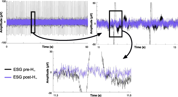
Figure 3. Filtering the cardiac artifact via adaptive filtering algorithm: A exemplary section of ESG data pre- filtering shown in black and post-
 filtering shown in blue at a time scale of (top left) 50 s, (top right) 2 s, (bottom) 200 ms with an amplitude scale of ± 100, 50, and 30 µV, respectively. The black square denotes where the data for the next plot, designated with the arrow, was derived.
Download figure:
Standard image High-resolution image3.2. K-means clustering
Figure 4 shows the results of the k-means clustering algorithm, which resulted in five clusters and 107 total dipoles. Figure 4 also shows the number of participants that make up each cluster, the number of IC sources per cluster, the Talairach coordinates, and the Brodmann area (BA) for the corresponding cluster. Talairach coordinates and BAs were identified from the Talairach atlas [38]. The BAs were searched within ± 5 mm cube ranges around each cluster centroid and the maximum distance from the centroid to the BA area was 3 mm.
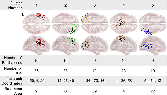
Figure 4. Clusters of equivalent dipole sources fit to independent components: Five clusters of dipoles were found across participants, trials, and conditions. Brodmann areas are the regions found within a ± 5 mm search range of the cluster centroids and had a maximum distance of 3 cm in this study. Cluster number is for referencing of individual cluster location in the text. The left side of the transverse view is denoted with a L on cluster 1.
Download figure:
Standard image High-resolution image3.3. ESG PSD analysis
Figure 5(A) demonstrates PSD changes during left and right knee flexion when compared to rest employing a bipolar configuration denoted by the line connecting sensors for a representative participant (NIS007). The data demonstrate a significant (p < 0.05) decrease in PSD during left and right knee flexion when compared to resting state. Changes are localized to the top half of the array (top left and right PSD plots) while the bottom half of the array had minimal changes. It should be noted that while several participants, including the one shown, had decreases in PSD during movement while compared to rest, others (n = 3) had increased PSD compared to rest. Further, in some cases the level of PSD change found (increase or decrease) was side specific (i.e. left vs. right). Additional examples of changes in PSD during knee flexion and plantarflexion can be found in the supplementary materials.
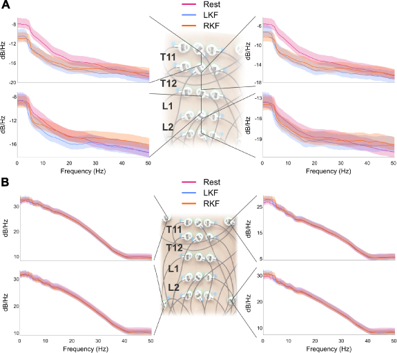
Figure 5. Power spectral density (PSD) changes during knee flexion: Average changes in PSD during right (RKF) and left knee flexion (LKF) when compared to control (Rest) (A) utilizing a bipolar configuration where the inferior sensor is subtracted from the superior and is denoted by the lines connecting sensors. Changes in PSD of the EKG sensors, or sensors placed around the array, (B) from the same participant (NIS007) and time period. Light shaded area represents the 95% confidence interval for that condition. Additional examples of PSD changes during knee flexion or plantarflexion can be found in the supplementary materials.
Download figure:
Standard image High-resolution imageAnalysis of the EKG sensors as seen in figure 5(B) for the top and bottom left and right of the array during the same time periods used for the analysis found minimal change in PSD during left or right knee flexion when compared to rest. Similar changes were found across participants with changes in the PSD during movement more prevalent during knee flexion than plantarflexion, however none of the changes found in the EKG sensors matched the pattern of changes seen in the ESG array.
3.4. Functional connectivity
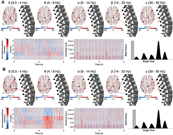
Figure 6 demonstrates the functional connectivity changes within the participant IC data and between the cluster data and ESG data using a two second window of time just prior to right plantarflexion execution figure 6(A) and a two second window of time during movement preparation and execution (B). Normalized amplitude data is shown for the clusters (bottom left) and ESG data (bottom middle), while the time window is shown using a gray box overlaid on the EMG data for the right soleus (bottom right). Data are for a representative participant and videos presenting gPDC over time can be found in the supplementary materials.
Figure 6. Functional connectivity changes over time: Significant differences in functional connectivity (gPDC) during right plantarflexion for a representative participant. Data shown are from a single block and organized by band (top) corresponding cluster data (bottom left) and ESG data (middle). The gray shaded area of the EMG data from the right soleus (bottom right) is the two second section of data being shown which is (A) just prior to first movement and (B) during first movement initiation. Cluster number location is shown in the delta band panel (top left). See supplementary materials for videos demonstrating changes in functional connectivity over time for both plantarflexion and knee flexion conditions.
Download figure:
Standard image High-resolution image
4. Discussion
In this study we identified five common clusters of EEG activity among ten neurologically intact participants. Specifically, BA 9 (cluster 1) has been shown to be involved with motor planning and working memory. BA 8 (cluster 2) has been demonstrated to be important for visual attention. BA 19 (cluster 3) is associated with processing visual information. BA 4 (cluster 4) is also known as the primary motor cortex and is responsible for execution of movements. BA 39 has been shown to play a role in spatial cognition, memory retrieval, and attention. Each cluster contained at least one IC from each participant, with the exception of one participant who did not have IC's that fell within the designated range for clusters 3 and 5.
This is the first study demonstrating the feasibility of high-density ESG to characterize single joint movements from changes in the electrical activity at the level of the spinal cord during movement. While caution must be taken in interpreting the results, we demonstrated that sensors placed bilaterally approximately 5 cm from midline at the top and bottom of the lumbar ESG array did not show changes in PSD during movement that were comparable with the analysis performed using the midline sensors in the array. The experiment was conducted in a controlled environment to minimize the possibility of sensor movement during the two tasks performed and, in most cases, the changes were localized within the array in the superior-inferior direction. Furthermore, it has been demonstrated that peripheral nerve stimulation can evoke a response from the spinal cord that can be recorded utilizing surface electrodes with only one paper known to the authors showing proof of concept for changes in surface recordings during movement using a similar methodology [13, 14].
Unfortunately, this study ultimately cannot conclude that the recorded signals originated from the spinal cord. Nevertheless, we found that the power spectral changes behave similarly to invasively recordings done using animal models. For example, it has been demonstrated that there is a decrease in 8–30 Hz activity recorded from the epidural space in the skull before and during forelimb movement in rats [39]. Another study recording activity from the lumbar spinal cord using micro wires found low frequencies (0.5–30 Hz) and high frequencies (100 Hz) conveyed more information about hind limb movement in cats [40]. Additionally, gPDC analysis suggests that the ESG recordings are bidirectional, which further reduces the likelihood that the data are from some other physiological source such as EMG which should cause mono-directional changes in gPDC (i.e. from a cluster location to the muscle being activated). Our findings suggest that the information provided by ESG is localized to the ESG array and provides useful information despite unknown origins.
There are several limitations to the study and one is due to the anatomical differences between individuals where the spinal cord can terminate up to two vertebral levels from the mean location, thus averaging the data was not best practice [41]. Future work could use MRI data to standardize locations between participants so that a group average could be performed, however even this may be challenging due to the anatomical differences of the vertebra and the conductivity of the tissues, which may need to be taken into account for this type of analysis. Nevertheless, individual variability in the patterns of ESG measurements are likely to have at least some diagnostic value.
Another limitation of the proposed noninvasive technique is that the ESG electrodes are well positioned to record mainly the posterior funiculus, which contains ascending pathways (dorsal column fibers) carrying information concerning touch and limb position from the body to the brain. Thus, the ESG technique seems less ideal to record descending motor information to the muscles. However, we suspect that some of these descending signals may be registered indirectly by the ESG electrodes via volume conduction, particularly prior to movement when the spinal cord may be 'quiet'. Interestingly, the gPDC findings (see figure 6(A), alpha band) shows significant changes in functional connectivity in alpha, beta and gamma bands directed from the brain to the spinal cord (that is, descending information) prior to movement. Conversely, gPDC changes directed from the spinal cord to the brain (i.e. ascending information) in the delta, beta and gamma bands are shown during the initial phases of movement (figure 6(B)). Future studies should use source analysis and an appropriate spinal cord model and lead field matrix to estimate the sources of these ESG signals within the spinal cord during volitional (self-initiated or attempted) lower-limb movements [42].
Due to the low conductivity of fatty tissues, we hypothesize that body composition is one of the largest limitations to the usefulness of ESG in adults and while this was not a factor in the participant selection for this study, the body composition of the participants was well within normal ranges [43].
Due to preparatory contraction of back muscles just prior to and during movement/postural adjustments, the experiments were performed in the prone position to minimize or eliminate the influence of muscle artifact contamination on the ESG signal. Further studies should be done to determine if ESG can be recorded in the sitting or standing positions, which would further expand uses for the recording modality. Additionally, while this experiment was performed using recordings over the approximate location of the lumbar enlargement during lower limb movements, future work with recordings over the approximate location of the cervical enlargement may be useful to determine if changes can be detected during arm and/or hand movement(s) and if different fine movements can be discriminated.
Another limitation is the low signal to noise ratio which was found to be at best similar to EEG and could be made worse due to SCI, which is thought to decrease the amplitude of spared descending signals [44]. However, previous work has demonstrated that transcranial magnetic stimulation in conjunction with voluntary effort can create motor evoked potentials that can be recorded on the surface of the skin over the spinal column above, at, and below the lesion in individuals who are motor and sensory complete (AIS A) [45]. This suggests that ESG recordings may provide useful information even for people with a SCI where the signal is degraded.
Future work will be done with people who have a SCI to determine if ESG is sensitive enough to detect changes in descending drive (i.e. attempting movement) or for measuring the resting state of the spinal cord after injury, which may provide valuable insights into adaptations made by the spinal cord and how to treat them. If validated, longitudinal studies could also be done with participants with an SCI while undergoing therapy to determine if ESG can be used as a metric for recovery.
5. Conclusion
In this study we utilized a combination of EEG, ESG, and EMG in neurologically intact participants (N = 10) while performing knee flexion or plantarflexion in the prone position. To the authors knowledge, this is the first time ESG has been utilized in this method and the first study demonstrating the feasibility of ESG to determine movement in neurologically intact participants. ESG was demonstrated to have localized changes in PSD during movement when compared to rest and these changes were not found with sensors placed bilaterally 5 cm from the top and bottom of the array. We then demonstrated bidirectional changes in functional connectivity (increases and decreases) during movement. The findings of this study could aid in uncovering fundamental knowledge about the intact spinal cord and how to better treat SCI.
Acknowledgments
This work was supported by The Institute for Rehabilitation and Research (TIRR) Mission Connect grant (Award # 021-112) The funders were not involved in the design of the study, the collection, analysis, and interpretation of the experimental data, the writing of this article, or the decision to submit this article for publication.
Data availability statement
Data is publicly available at https://ieee-dataport.org/documents/dataset-electrospinography-esg-non-invasively-recording-spinal-sensorimotor-networks.
CRediT authorship contribution statement
Alexander G Steele: Conceptualization, Data Acquisition, Methodology, Software Programming, Formal analysis, Data Curation, Writing—Original draft. Amir H Faraji: Conceptualization, Funding acquisition, Methodology, and Writing—review & editing. Jose L Contreras-Vidal: Conceptualization, Funding acquisition, Methodology, Resources, Supervision, Visualization, EEG Analysis Strategy, and Writing—review & editing. All authors have reviewed and approved the manuscript.
Supplementary data (4.2 MB MP4)
Supplementary data (4.3 MB MP4)
Supplementary data (4.2 MB MP4)
Supplementary data (4.3 MB MP4)
Supplementary data (4.3 MB MP4)
Supplementary data (2.4 MB MP4)
Supplementary data (2.4 MB MP4)
Supplementary data (2.4 MB MP4)
Supplementary data (2.4 MB MP4)
Supplementary data (2.4 MB MP4)
Supplementary data (2.8 MB PDF)