Abstract
We study the environment of radio galaxies with different morphological types using the Proctor sample, which was built from the Faint Images of the Radio Sky at Twenty-Centimeters (FIRST) survey archive. Among the 15 radio galaxy types classified by Proctor, 199 C-shaped (i.e., wide- or narrow-angle tail) and 203 S-shaped (i.e., S- or Z-shaped) sources are selected in this work, which are located in the redshift range of 0.02 < z < 1, because these two subsamples are relatively larger than the other subsamples in the Proctor sample. By cross-matching these radio galaxies with the optical sources drawn from the Sloan Digital Sky Survey (SDSS) database and counting the SDSS sources with an r-band absolute magnitude brighter than −19 located within a 0.5 Mpc distance around each source (i.e., the richness), we find that the fraction of C-shaped sources with a richness above 10 is larger than that of S-shaped sources. We have also correlated the radio galaxies in our sample with the brightest cluster galaxies (BCGs) defined in the NASA/IPAC Extragalactic Database (NED), and infer that the C-shaped sources are more likely to be BCGs than the S-shaped sources. These results support the idea that C-shaped radio galaxies often reside in a richer environment than radio galaxies with other morphological types.
Export citation and abstract BibTeX RIS
1. Introduction
The emissions of radio galaxies exhibit various morphologies, which may result from different host galaxy conditions or ambient environment, e.g., the size of the host galaxy (e.g., Miraghaei & Best 2017), the black hole to stellar mass ratio (e.g., Miraghaei & Best 2017), the motion of the central black hole (e.g., Florido et al. 1990), the intra-cluster medium (ICM) density (e.g., Begelman et al. 1984) and the environmental galaxy richness (e.g., Wing & Blanton 2011), i.e., a count of magnitude limited galaxies within a certain distance from the target source. Basically, there are two primary morphological classes of radio galaxies: Fanaroff-Riley type I and type II (FR I and FR II respectively; Fanaroff & Riley 1974). Typically, FR Is show a decreasing radio flux density at the plumes as the distance from the core increases, and FR IIs exhibit an inverse tendency with two bright hotspots at each end of the radio lobes.
Except for this rough classification, more complicated morphological taxonomies have been introduced in previous studies, including types such as wide- or narrow-angle tail sources (WATs or NATs respectively; e.g., Rudnick & Owen 1976), S- or Z-shaped sources (e.g., Florido et al. 1990), X-shaped sources (e.g., Leahy & Parma 1992; Cheung 2007), ring-like sources (e.g., Buta & Combes 1996), double-double sources that consist of two pairs of lobes with a common center (e.g., Schoenmakers et al. 2000a; Kaiser et al. 2000; Schoenmakers et al. 2000b) and others (e.g., hybrid morphology radio sources; Rudnick & Owen 1976).
In this work, we investigate the relationship between morphology and environment of radio galaxies. Only the C-shaped (i.e., WATs or NATs) and S-shaped (i.e., S- or Z-shaped) morphological types with sufficient sources that possess the highest fractions (21% and 20%, respectively) in a certain Proctor sample (Proctor 2011) classification are selected as our targets. The C-shaped morphology is thought to be a direct result of ram pressure exerted on the jets when both the ICM density and relative velocity between the radio galaxy and ambient gas are high enough (Owen & Rudnick 1976; Eilek et al. 1984; Burns 1990; Ball et al. 1993; Bliton et al. 1998). The S-shaped morphology may be caused by a precessional central black hole, which causes changes in the orientation of the radio jet (Gower et al. 1982). The precession of the central black hole may be produced by the presence of a tilted accretion disk (Lu 1990; Lu & Zhou 2005), or another black hole in the same nucleus Begelman et al. 1980. Because of the complex conditions that result in various morphologies, details on the formation of different morphological types of radio galaxies still need more investigation.
In order to study the impact of the environment on morphology, Zirbel (1997) studied the environment of FR sources and found that FR Is tend to reside in richer groups than FR IIs. By counting the number of galaxies with the Sloan Digital Sky Survey (SDSS) absolute r magnitude Mr > −19 within a radius of 1 Mpc around each radio source, and calculating the statistics of the richness distribution of the sources, Wing & Blanton (2011) confirmed that bent radio sources are more often found in richer clusters than non-bent radio sources. Miraghaei & Best (2017) investigated the properties of the host galaxies and environment, and found that compared with normal FR radio sources, the radio luminosity and host galaxy size of WATs are smaller, and the WATs tend to reside in denser regions than double-double and FR hybrid sources. The environment generally includes the ICM properties and richness; in this work, we choose to use the richness to indicate the environment.
This paper is organized as follows. In Section 2, we construct the sample and describe how to determine the optical counterparts of radio galaxies. Section 3 presents measurement of the richness around each radio source. In Section 4, we cross-match our sources with the brightest cluster galaxies (BCGs) using five galaxy cluster catalogs to determine the BCG proportions of the C- and S-shaped radio galaxies in our sample. In Section 5, we study physical properties of the radio galaxies. A brief summary is provided in Section 6. The ΛCDM cosmology with H0 = 70 km s−1 Mpc−1, ΩΛ = 0.7 and Ωm = 0.3 is adopted in this paper.
2. Sample Construction
2.1. Selection of Radio Galaxies
The Faint Images of the Radio Sky at Twenty-Centimeters (FIRST) survey covers over 10 000 square degrees of the sky that overlaps the SDSS area, with a flux density threshold of 1 mJy and a resolution of 5''. Radio galaxies in FIRST have been classified into 15 types by Proctor (2011) according to their morphology. We use the 412 C-shaped sources and 400 S-shaped sources that belong to the Proctor sample to construct the initial sample for our research.
2.2. Optical Counterparts
Optical sources in the SDSS Data Release 14 (DR14) (Abolfathi et al. 2018) are used for cross-matching the radio sources. Following the procedure presented in Wing & Blanton (2011), we first match each galaxy in our sample with the SDSS sources within a separation of 10''. The number of cross-matched radio sources of the two subsamples is set as a function of separation. Wrong cross-matchings could exist, because the projection of unrelated optical sources may be located within a small separation from the radio galaxies. To estimate the wrong matches, we shift both the right ascension (R.A.) and declination (Dec.) of each radio source by adding 30'; all the shifted coordinates will be physically unrelated to their former SDSS counterparts. Then we match the shifted coordinates with the SDSS sources as in previous steps to achieve random matches at different matching separations. The random matches are not real radio-optical counterparts, but give an estimation of possible wrong matches at each separation. The number of random matches is also set as a function of the separation between counterparts.
The upper and lower panels in Figure 1 illustrate cross-matching procedures for the C-shaped and S-shaped sources, respectively, and the left panels show the cross-matched number as a function of separation. Both of the real matches display peaks appearing below a separation of 1'', but the random matches increase slowly as the separation increases, which is the result of the increasing cross-matching area as the separation increases. In the right panels, the solid lines signify the cumulative real matches corresponding to the left panels, as a function of separation. The dot-dashed lines represent cumulative good matches, which are the cumulative real matches minus the cumulative random matches, as a function of separation. The dashed lines indicate the matching reliability of the subsamples, which is the value of cumulative good matches divided by cumulative real matches. We expect a 90% reliability cutoff, which corresponds to a separation of about 3.3'' for C-shaped sources and 4.2'' for S-shaped sources. So, the matching separation limits of 3.3'' and 4.2'' are determined for the C-shaped and S-shaped subsamples, respectively. Finally, the sample contains 199 C-shaped sources and 203 S-shaped sources in the redshift range 0.02 < z < 1 after the cross-matching steps. The sources are listed in Table 1.

Fig. 1 The upper and lower panels illustrate cross-matching procedures of the C-shaped and S-shaped sources, respectively. In the left panels, the solid line histograms represent the number of C-shaped or S-shaped radio-optical matches, as a function of separation. The dashed line histograms mean distributions of random matches for the shifted subsamples. In the right panels, the solid lines show the cumulative matches of C-shaped or S-shaped sources, as a function of separation. The dot-dashed lines correspond to cumulative good matches that are the cumulative real matches minus the cumulative random matches. The dashed lines signify the percentage of true matches.
Download figure:
Standard imageTable 1. The Sample
| Name | R.A. (J2000) | Dec. (J2000) | Redshift | Type | mr (mag) | Mr (mag) | log10(L1.4 G) (W Hz−1) | Extent (Mpc) |  |
fc | GClstr |
|---|---|---|---|---|---|---|---|---|---|---|---|
| (1) | (2) | (3) | (4) | (5) | (6) | (7) | (8) | (9) | (10) | (11) | (12) |
| J000330.7+002756 | 00h03m30.73s | +00d27m56.0s | 0.19199S | C | 17.07 | −22.93 | 24.62 | 0.17 | 21 | 1.00 | WHL |
| J002216.5+010403 | 00h22m16.56s | +01d04m03.2s | 0.53402S | S | 20.30 | −23.21 | 25.59 | 0.18 | −1 | 1.49 | |
| J003432.6−093444 | 00h34m32.61s | −09d34m44.5s | 0.46118P | S | 19.93 | −22.86 | 25.21 | 0.09 | 4 | 1.28 | |
| J004152.1+002837 | 00h41m52.10s | +00d28m37.3s | 0.15199S | C | 16.46 | −22.87 | 24.79 | 0.11 | 25 | 1.00 | WHL |
| J010236.5−005007 | 01h02m36.57s | −00d50m07.6s | 0.24331S | C | 17.65 | −22.97 | 24.96 | 0.11 | 29 | 1.00 | RM |
| J010242.4−005032 | 01h02m42.42s | −00d50m32.9s | 0.24281S | C | 17.64 | −22.99 | 25.18 | 0.19 | 24 | 1.00 | WHL |
| J010403.0−002440 | 01h04m03.04s | −00d24m40.9s | 0.28307S | C | 17.90 | −23.23 | 25.52 | 0.22 | 19 | 1.00 | |
| J011425.5+002932 | 01h14m25.59s | +00d29m32.5s | 0.35461S | C | 18.45 | −23.32 | 25.60 | 0.19 | 19 | 1.07 | WHL |
| J012947.0+004633 | 01h29m47.03s | +00d46m33.4s | 0.42151P | C | 21.01 | −21.80 | 25.51 | 0.21 | −1 | 1.19 | |
| J013247.1+011545 | 01h32m47.16s | +01d15m45.4s | 0.12560S | C | 15.16 | −23.68 | 24.99 | 0.14 | 48 | 1.00 | WHL |
| J020613.2−021504 | 02h06m13.27s | −02d15m04.6s | 0.34877P | S | 19.42 | −22.26 | 25.00 | 0.11 | 10 | 1.06 | |
| J021534.3−032202 | 02h15m34.36s | −03d22m02.7s | 0.76463P | S | 22.74 | −22.24 | 26.47 | 0.24 | −11 | 2.84 | |
| J021619.7−024433 | 02h16m19.75s | −02d44m33.5s | 0.06952S | C | 14.97 | −22.43 | 24.56 | 0.10 | 17 | 1.00 | WHL |
| J024558.4−064859 | 02h45m58.45s | −06d48m59.9s | 0.13857S | C | 16.52 | −22.58 | 24.78 | 0.14 | 28 | 1.00 | |
| J024612.8−084735 | 02h46m12.81s | −08d47m35.8s | 0.13816S | C | 16.52 | −22.58 | 24.83 | 0.13 | 16 | 1.00 | |
| J031147.3+010846 | 03h11m47.36s | +01d08m46.6s | 0.21192S | C | 18.54 | −21.98 | 24.42 | 0.10 | 23 | 1.00 | |
| J031357.1−001531 | 03h13m57.13s | −00d15m31.2s | 0.31706S | S | 18.62 | −22.93 | 25.26 | 0.16 | 5 | 1.02 | |
| J071501.6+404820 | 07h15m01.68s | +40d48m20.3s | 0.51359P | S | 21.51 | −21.59 | 25.55 | 0.17 | 10 | 1.42 | |
| J072725.1+310934 | 07h27m25.14s | +31d09m34.6s | 0.24987P | C | 18.41 | −22.37 | 25.92 | 0.35 | 28 | 1.00 | |
| J073202.4+274530 | 07h32m02.41s | +27d45m30.9s | 0.36894P | S | 19.27 | −22.70 | 25.26 | 0.20 | 11 | 1.09 | |
| J073229.7+374420 | 07h32m29.76s | +37d44m20.1s | 0.20121S | C | 17.49 | −22.68 | 24.84 | 0.08 | 49 | 1.00 | GMBCG |
| J073441.9+361129 | 07h34m41.93s | +36d11m29.5s | 0.43209S | C | 19.60 | −22.98 | 25.50 | 0.16 | 5 | 1.21 | WHL |
| J073539.8+251020 | 07h35m39.80s | +25d10m20.3s | 0.07873P | C | 15.10 | −22.64 | 24.38 | 0.09 | 18 | 1.00 | WHL |
| J073540.4+361912 | 07h35m40.47s | +36d19m12.7s | 0.12015P | C | 16.47 | −22.31 | 24.45 | 0.03 | 35 | 1.00 | |
| J073618.0+241043 | 07h36m18.00s | +24d10m43.9s | 0.14710S | C | 16.39 | −22.93 | 25.39 | 0.17 | 46 | 1.00 | WHL |
| J073837.7+482046 | 07h38m37.74s | +48d20m46.7s | 0.09523P | S | 15.75 | −22.56 | 23.74 | 0.03 | 6 | 1.00 | |
| J074041.9+345843 | 07h40m41.95s | +34d58m43.3s | 0.57113S | S | 20.10 | −23.87 | 25.58 | 0.35 | 0 | 1.62 | |
| J074115.4+163254 | 07h41m15.49s | +16d32m54.1s | 0.10132S | C | 16.17 | −22.15 | 23.68 | 0.05 | 69 | 1.00 | |
| J074118.0+163156 | 07h41m18.02s | +16d31m56.8s | 0.10029P | C | 15.75 | −22.55 | 23.86 | 0.08 | 70 | 1.00 | WHL |
| J074143.0+174056 | 07h41m43.04s | +17d40m56.9s | 0.12360P | C | 16.07 | −22.76 | 24.53 | 0.15 | 11 | 1.00 |
The full table is online at http://www.raa-journal.org/docs/Supp/ms4370table1.pdf.
3. Richness of the Selected Radio Galaxies
3.1. Definition of Richness
We choose the richness measurement system similar to those adopted in the previous works (Allington-Smith et al. 1993; Zirbel 1997; Blanton et al. 2000), where the richness  represents the number of galaxies with absolute visual magnitude MV > −19 within a 0.5 Mpc distance around a radio galaxy. Since we draw data from SDSS catalogs, the SDSS r-band absolute magnitude is adopted, and the richness
  is defined as the number of galaxies brighter than Mr = −19 within a 0.5 Mpc radius circle centered on a radio galaxy.
3.2. Background Galaxy Density
To estimate the richness, the background galaxies should be subtracted from the total number counts within the 0.5 Mpc circle. The large number of sources in the SDSS field of view provides us with an approach for counting background galaxies. We use the spectroscopic redshift whenever it is available, otherwise, the photometric redshift is used. For a small fraction of sources with no redshift information in SDSS DR14, the redshifts in DR8 (Aihara et al. 2011) are adopted. The k-corrections are calculated following the method provided in Blanton & Roweis (2007), and the extinctions in the SDSS catalog are also considered to correct the absolute magnitudes (Schlegel et al. 1998).
We follow the procedure provided in Wing & Blanton (2011) to count galaxies brighter than Mr = −19 within an annulus whose inner and outer radii are 2.7 Mpc and 3 Mpc, respectively, centered on the core of each radio source. Most galaxies located in this distant annulus are expected to be unassociated with the potential cluster (Wing & Blanton 2011). The galaxy density within the annulus is set as the background density, which should be subtracted from the total density derived within the 0.5 Mpc radius circle. The richness  is obtained by multiplying the area within the 0.5 Mpc circle and the subtracted galaxy density.
3.3. Schechter Correction
The limiting SDSS r-band magnitude is mr ∼ 22, since sources with absolute magnitude Mr = −19 cannot be detected above redshift z ∼ 0.3. Thus the richness we obtain from the previous steps may be smaller than the real one. In order to estimate the richness around the higher redshift sources, the raw richness should be multiplied by a Schechter correction factor to give a corrected richness measurement (Hill & Lilly 1991; Zirbel 1997; Blanton et al. 2000; Wing & Blanton 2011). According to Wing & Blanton (2011), the correction factor is defined as

where ϕ(M) is the integrated Schechter luminosity function, which predicts the number of expected galaxies brighter than a given magnitude (Schechter 1976), Mr = −19 represents the faint end of absolute magnitude in the richness definition and Mr,lim denotes the absolute magnitude corresponding to the limiting SDSS magnitude (mr ∼ 22) at the redshift of the target source. The correction factor calculated by the mean Schechter luminosity function may be a little rough for the radio sources located in galaxy clusters. We adopt the Schechter luminosity function with parameters  and α = −1.26, based on the results of Montero-Dorta & Prada (2009). When the sources in our sample have redshifts below z ∼ 0.3, all galaxies at those redshifts with absolute magnitudes brighter than Mr = −19 could be detected even at the limiting magnitude of SDSS, and thus the correction factor is set as fc = 1.
3.4. Richness Measurement and Results
After the Schechter correction is applied, we obtain the richness around the radio sources. Figure 2 shows the fraction of sources as a function of richness. We find that when the richness  , the cumulative fraction of C-shaped sources is 82.9%, which is larger than 46.3% of the S-shaped ones. We define galaxies with richness
  as residing in a poor environment. When
  1, the fraction of C-shaped sources is 6.0% and it is 23.2% for S-shaped sources. The average richness is
  for the C-shaped sources, and
  for S-shaped ones (Fig. 2). Using the Kolmogorov-Smirnov (K-S) test, we examine the likelihood of the richness distribution for the C-shaped and S-shaped subsamples being identical, and find that the P value is 2.47 × 10⁻¹⁷%. Therefore, compared with S-shaped sources, C-shaped ones are significantly more likely to be located in a richer environment. Four examples of C-shaped and S-shaped sources and their environments are shown in Figures 3 and 4 respectively.

Fig. 2 The fraction of sources as a function of richness for the C- and S-shaped sources. The solid line histogram represents C-shaped sources and the dashed line histogram signifies S-shaped sources.
Download figure:
Standard image
Fig. 3 FIRST contours and SDSS r-band images. The radio emission maps are square root scaled with four contours, with minimum contours of 0.5 mJy and maximum contours of 3.4 mJy and 36.6 mJy for the upper and lower panels, respectively. The circles centered on the sources with 0.5 Mpc radius are shown in the left panels, and the corresponding centered 0.5 × 0.5 Mpc areas are displayed in the right panels. The top panels feature a C-shaped source located at redshift z = 0.197 with  . The bottom panels depict a C-shaped source located at redshift z = 0.209 with
  .
.
Download figure:
Standard image
Fig. 4 FIRST contours and SDSS r-band images. The radio emission maps are square root scaled with four contours, with minimum contours of 0.5 mJy and maximum contours of 1.7 mJy and 6.3 mJy for the upper and lower panels, respectively. The circles centered on the sources with 0.5 Mpc radius are shown in the left panels, and the corresponding centered 0.5 × 0.5 Mpc areas are displayed in the right panels. The top panels feature an S-shaped source located at redshift z = 0.353 with  . The bottom panels depict an S-shaped source located at redshift z = 0.083 with
  .
.
Download figure:
Standard imageWe compare this result with that of Wing & Blanton (2011) in which the C-shaped radio galaxies are denoted as bent sources with multiple-components. Most bent sources used in that paper are not certainly classified as C-shaped sources in the Proctor sample, but are given a probability of being bent, e.g., the source J075718.7+345905 with a probability of 2% of being bent in the Proctor sample is treated as a bent source in Wing & Blanton (2011). About 71% of bent radio galaxies reside in a cluster environment, while the fraction is 44% for non-bent sources (Wing & Blanton 2011). Therefore, both Wing & Blanton (2011) and our results support the idea that bent radio galaxies often reside in richer environments than non-bent radio sources.
4. Correlation Between a Radio Source and the Corresponding BCG
As another way to investigate the environmental differences between C-shaped and S-shaped radio galaxies, we investigate the proportion of sources that are BCGs in the galaxy clusters.
We cross-match the radio sources with the BCGs in all sample clusters, which are defined using data from the NASA/IPAC Extragalactic Database (NED) with an offset of 3''. The cross-matched BCG catalogs include the WHL (Wen et al. 2009), Gaussian Mixture Brightest Cluster Galaxy (GMBCG; Hao et al. 2010), MaxBCG (Koester et al. 2007), [EAD2007] (Estrada et al. 2007) and redMaPPer (RM; Rozo et al. 2015). We find that 51.8% (103 out of 199) of C-shaped radio sources have BCG identities, but only 15.8% (32 out of 203) of S-shaped sources are BCGs. Thus the C-shaped sources are more likely to be the BCGs of galaxy clusters than the S-shaped sources. This is not only consistent with the result in Section 3 that C-shaped sources often reside in a richer environment than S-shaped sources, but also confirms the idea that C-shaped radio galaxies are usually associated with the corresponding BCGs (Burns 1981).
Nearly all sources with BCG identities have positive richness values, except for the three C-shaped galaxies, J080611.3+253138, J102228.2+165315 and J145022.4+272820. J080611.3+253138 is a source in the MaxBCG catalog at redshift z ∼ 0.17, possibly because the richness definition used by Koester et al. (2007) to search for BCGs (i.e., the number of sources brighter than 0.4L* in the SDSS i-band within a radius of R200) is different from ours. It is the same case with the other two BCG sources (J102228.2+165315 and J145022.4+272820) having negative richness values. Note that a galaxy cluster included in one catalog may not be included in another one due to different richness definitions (e.g., the galaxy J080611.3+253138, the poorest cluster whose richness is 10 in the MaxBCG catalog, is unrelated to the cluster in the GMBCG catalog).
We summarize our results in Table 1, where the source names are shown in column 1, the R.A. and Dec. of the sources in J2000 coordinates in columns 2 and 3 respectively, the redshift of the sources (with the superscripts S for spectroscopic redshift and P for photometric redshift) in column 4, the types of source (C for C-shaped and S for S-shaped) in column 5, the SDSS r-band magnitude of the sources in column 6, the r-band absolute magnitude in column 7, the radio luminosity in 1.4 GHz in column 8, the radio source extent (see the text for the definition) in column 9, the richness in column 10, the correction factors in column 11 and the catalogs of the cross-matched BCGs in column 12.
5. Physical Properties of C-Shaped and S-Shaped Radio Sources
We investigate the physical properties of the sources, such as whether or not radio source extent and luminosity are correlated with richness. The radio source extent of the galaxies is defined as the projected distance between the core and the farthest edge of lobes or plumes in the FIRST images. Figure 5 shows the relationship between richness and source extent of the galaxies. The radio source extent of most galaxies is smaller than 0.5 Mpc, the scale used to calculate the richness. Four giant S-shaped radio galaxies (J083448.7+173651, J135517.6+292333, J141621.7+590032 and J160420.0+373117), whose source extents are larger than 0.5 Mpc, reside in a poor environment with  , and two giant C-shaped radio galaxies (J124619.2+262635 and J155806.8+451955) reside in a richer environment with richness
  . All radio galaxies with richness
  possess a source extent smaller than 0.3 Mpc, i.e., radio sources that are located in a very rich environment tend to exhibit small sizes, a tendency that is more obvious for the C-shaped sources as shown in Figure 5.
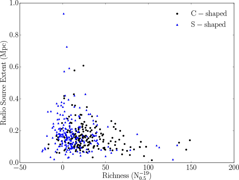
Fig. 5 Richness vs. radio source extent. The triangle symbols represent S-shaped sources and the circle symbols C-shaped sources.
Download figure:
Standard imageThe 1.4 GHz radio luminosities of the sources are also calculated using the radio flux densities from the catalog of Condon et al. (1998). Figure 6 illustrates the radio luminosities of the sources against the richness. There is no obvious correlation between radio luminosity and richness, which agrees with the conclusion of Zirbel (1997).

Fig. 6 Relationship between richness and radio luminosity at 1.4 GHz of the radio sources. The symbols are the same as in Fig. 5.
Download figure:
Standard image6. Summary
We have selected C-shaped and S-shaped radio galaxies from the Proctor sample and cross-matched them with SDSS sources. Then we calculated the richness around each source to study differences in the environment between C-shaped and S-shaped radio galaxies. Moreover, the correlation between these radio galaxies and the BCGs has been investigated. Based on these results, we draw the conclusions that the fraction of C-shaped sources with richness  is 82.9%, which is significantly larger than 46.3% for S-shaped sources. That is, C-shaped sources tend to be located in richer environments than S-shaped sources. About 51.8% of C-shaped sources are the BCGs of galaxy clusters, which is larger than 15.8% of S-shaped sources with BCG identities. Enlargement of the two subsamples will be helpful for confirming the conclusions and providing a better understanding of the relationship between the morphologies of radio galaxies and their surrounding environments.
Acknowledgements
We thank the reviewer and editor for their useful comments that have helped to greatly improve the manuscript. This work is supported by the Ministry of Science and Technology of China (Grant Nos. 2018YFA0404601 and 2017YFF0210903), and the National Natural Science Foundation of China (Grant Nos. 11433002, 11621303, 11835009 and 61371147).
Footnotes
- 1
Negative values of richness indicate that within 0.5 Mpc from the radio galaxies, the local galaxy density is lower than the background galaxy density (Wing & Blanton 2011).