
Abstract
Isovector neutron-proton (np) pairing and particle-number fluctuation effects on the spectroscopic factors (SF) corresponding to one-pair like-particle transfer reactions in proton-rich even-even nuclei are studied. With this aim, expressions of the SF corresponding to two-neutron stripping and two-proton pick-up reactions, which take into account the isovector np pairing effect, are established within the generalized BCS approach, using a schematic definition proposed by Chasman. Expressions of the same SF which strictly conserve the particle number are also established within the Sharp-BCS (SBCS) discrete projection method. In both cases, it is shown that these expressions generalize those obtained when only the pairing between like particles is considered. First, the formalism is tested within the Richardson schematic model. Second, it is applied to study even-even proton-rich nuclei using the single-particle energies of a Woods-Saxon mean-field. In both cases, it is shown that the np pairing effect and the particle-number projection effect on the SF values are important, particularly in N = Z nuclei, and must then be taken into account.
Export citation and abstract BibTeX RIS
1. Introduction
Due to the development of new experimental facilities, and in particular radioactive ion beam technology, it has become possible, during the last two decades, to produce and study nuclei close to the drip-lines [1–4]. The study of the structure of proton-rich nuclei has thus become a popular field of interest. As a result, the study of neutron-proton (np) pairing correlations has attracted lots of attention (see e.g. Refs. [5–15], for a review; see also Refs. [16] and [17]). Indeed, in N ≃ Z nuclei, the valence neutrons and protons occupy the same energy levels and, therefore, np pairing correlations are expected to play an important role. There are, in principle, two forms of np pairing correlations, i.e., the isovector (T=1) pairing, and the isoscalar pairing (T=0). For simplicity, in the present work we will consider only isovector pairing correlations.
The simplest way to treat isovector pairing correlations, in addition to the pairing between like-particle correlations, is the Bardeen-Cooper-Schrieffer (BCS) approach [18], extended to the np pairing case [19–28]. However, it is well known that the BCS approach breaks particle-number conservation symmetry [29, 30], either in the case of pairing between like-particles, or in the np pairing case. The particle-number fluctuations may affect predictions dealing with several observables, such as the moment of inertia [31–33], the two-neutron [34] or two-proton [35] separation energies, the nuclear radii [36, 37], the electromagnetic moments [38, 39], the pairing energy [40–42] or the beta transition probabilities [43, 44].
A rigorous treatment of the pairing correlations thus necessitates the restoration of the broken symmetry. Several methods have been used with this aim, including the Lipkin-Nogami method [45–49], which enables one to approximately conserve the particle number. Another approach consists of projecting onto the good particle number [29], either after the variation (methods of projected BCS (PBCS) type) [50–55] or after it (methods of fixed BCS (FBCS) type) [56–61]. In the case of the np pairing, a simultaneous projection on the isospin and the particle number may also be performed [62]. The higher Tamm-Dancoff approximation has also been used in order to treat the same problem [63–65].
Among the methods used in order to include the pairing correlations in a rigorous way, there is also the variation after mean field projection in realistic model spaces (VAMPIR) [66–68], as well as the variational approach [69, 70]. An alternative approach is to use a numerically exact technique to calculate pairing correlation energies at fixed particle number by employing the configuration-space Monte Carlo algorithm [71].
The recently proposed density matrix method [72, 73] also enables one to overcome the particle-number fluctuations that are inherent to the BCS approach. Let us also cite the nucleon pair approximation [74–76], as well as the generalized seniority [77, 78].
Another way to overcome the violation of particle number conservation is to use the shell-model-like approach in which the pairing Hamiltonian is diagonalized directly in the multiparticle configuration space [79].
In the present work, we will use the Sharp-BCS (SBCS) particle-number projection method [51, 53] which is of PBCS type and has the advantage of being not only exact but also discrete and hence easy to use numerically.
The spectroscopic factors (SF) were introduced fifty years ago in the theory of nuclear structure reactions to establish a relationship between nuclear reactions and structure [80]. Indeed, the SF provides a useful basis for the comparison either between theory and experiments or between theoretical models [81, 82]. The SF may be evaluated, e.g., in the study of knockout or stripping reactions. The study of the interactions with and between the transferred nucleons enables one to deduce information about the nature and occupancy of the single-particle orbits [83]. This quantity has thus been the object of many studies. On the experimental side, several procedures for a systematic extraction of the SF from various reactions have been proposed and applied (see e.g., Refs. [84–91]). Let us, however, cite Ref. [92], which discusses the role of SF extracted from transfer reactions in revealing neutron-proton correlation effects in nuclei.
Much effort has also been devoted to the study of the SF on the theoretical side. Among others, Hess et al. [93] proposed a method for the parametrization of the SF within the SU(3) shell model for light nuclei, and Timofeyuk [80, 94] calculated the SF using the inhomogeneous equation approach. Let us also cite Jensen et al. [81], who developed tools to compute spectroscopic factors within the coupled-cluster method and applied them to the nucleus 16O, as well as Fortune and Sherr [95], who extracted the SF for the 2+ decay using computed single-particle widths in the nucleus 21O. Gnezdilov et al. [96] calculated the total single-particle SF for some doubly magic and semi-magic nuclei within the self-consistent theory of finite Fermi systems. A more sophisticated method has been recently used by Srivastava and Kumar [83], who performed calculations of the SF strengths for the one-proton and one-neutron pick-up reactions 27Al(d,t)26 using ab initio approaches.
If the pairing correlations must be taken into account, a simple way to include them in the SF is the BCS method and its variants. One of the first works where the pairing between like-particles was taken into account in the evaluation of the SF is that of Baranger and Kuo [97], who used the BCS-TDA approximation. Aberg et al. [98] as well as C. Basu [99] also used the BCS approach. They respectively calculate the FS of spherical ground-state proton emitters and those of two-proton emitting nuclei. In order to study proton radioactivity, Yao et al. [100], as well as Zhang et al. [101] obtained the spectroscopic factor by combining the relativistic mean field theory with the BCS method. For their part, Kumar et al. [102] included the pairing correlations in the calculation of the proton SF of Sm isotopes using the pairing-plus-quadrupole model. However, in all these works, neither the particle-number fluctuations, which are inherent to the BCS approach, nor the np pairing correlations were taken into account. In a previous paper [103], the present authors studied the particle-number projection effect on the SF for one-pair of like-nucleon transfer reactions within a schematic model. However, only the like-particle pairing was taken into account. The aim of the present work is to study both isovector np pairing and particle-number fluctuation effects on the SF corresponding to one-pair like-particle transfer reactions in proton-rich even-even nuclei.
The paper is organized as follows. New expressions of SF corresponding to two-neutron stripping and two-proton pick-up reactions, taking into account the np pairing correlations, are established in Section 2, within the generalized BCS approach, either before or after the projection. Numerical results are presented and discussed in Section 3. They first deal with the schematic Richardson model. Even-even proton-rich nuclei are then considered using the single-particle energies of the Woods-Saxon model. The main conclusions are summarized in last section.
2. Formalism
2.1. Hamiltonian diagonalization - wave functions
Let us consider a system of N = 2Pn neutrons and Z = 2Pp protons in which the neutrons and the protons are assumed to occupy the same energy levels. It can be described, in the isovector pairing case, by the following total Hamiltonian [8, 9]
where t corresponds to the isospin component (t=n,p), and  (
( ) denotes the creation (annihilation) operator of a nucleon of type t in the |νt⟩ state, of energy
  .
.  is the time-reversed of the state |νt⟩. Gtt' is the pairing-strength, which is assumed to be constant. One also assumes that Gpn = Gnp.
H is diagonalized using the generalized Bogoliubov-Valatin transformation [7, 8]
where  is the quasiparticle (qp) creation operator and τ is the qp type.
The BCS ground-state |ψ⟩ is defined as the vacuum of the qp representation, i.e.,

This state may be also written in the particle representation by means of the Bogoliubov-Valatin transformation (2). One then has [53]
where we set
and

The coefficients  are defined by

with

K being the normalization constant given by
The pairing gap parameters are defined by
As the wave function (4) does not conserve the particle-number, it is necessary to perform a particle-number projection. In the present paper, we use the Sharp-BCS (SBCS) method [53]. In that method, the projected ground-state is given by
with
where we set
and
m,m' respectively refer to the projection order on the good neutron and proton numbers, and  means the summation over the same terms where
  is replaced by
  , then by
  and finally by
The normalization constant Cmm' is deduced from the condition
where we set
It is worth noticing that the following property, which is valid for any operator  which conserves the particle-number,

has been used in order to derive Eq. (15).
As soon as
|ψmm'⟩ converges towards the state with the good neutron and proton numbers.
Let us note that the state (11) can only describe even-even systems. This is the reason why in the present work we consider only one-pair like-particle transfer reactions in even-even systems.
2.2. Spectroscopic factors
In the present work, we use the schematic definition of the SF proposed by Chasman [104]. In the case of the transfer of one pair of paired like particles, the SF for a stripping reaction (denoted  (
t = n, p)) is given by
(
t = n, p)) is given by
The SF corresponding to a pick-up reaction (denoted  (t = n, p)) is given by
In these expressions, |ψi(A)⟩ and |ψf(A±2)⟩ respectively correspond to the wave functions of the initial (i) and final (f) states of the studied nucleus, A being the total number of nucleons in the initial state.
2.2.1. Before projection
Before the projection, the wave-functions are given by Eq. (4). The previous expressions of the SF then become
where

and


In the latter expressions, one just has to invert n and p to obtain the factors which appear in the expressions of  and
and  . When the np pairing effects vanish, i.e., when the np pairing gap parameter Δnp goes to zero, one has
which correspond to the expressions obtained in the pairing between like particles given by Eqs. (A8) and (A9), that is


In what follows, the notation stt (i.e., using lower case characters) will be reserved for the pairing between like particles.
2.2.2. After projection
After the projection, the wave-functions are given by Eq. (11). The SF may then be evaluated using the property (17). One then has


where t=n,p. After some algebra, one obtains


where
and


In the latter expressions, one just has to invert n and p as well as zk and zk' to obtain the factors which appear in the expressions of  and
and  . One notices a formal similarity between Eqs. (32)–(33) and Eqs. (21)–(22). Moreover, when the np pairing effects vanish, one has, assuming that m=m',


where t=n,p. This means that at the limit when Δnp goes to zero, the SF correspond to those obtained in the pairing between like particles, i.e.,


3. Numerical results- discussion
Calculations have been performed first within the schematic Richardson model [105]. This model is introduced here as a toy model in order to gain a better understanding of the dependence of the SF as a function of the various parameters. Let us note that the Richardson model is often used in order to compare the results with exact solutions. However, it enables one only to obtain the exact values of the energies but not the wave-functions that are needed in the calculation of the SF.
Even-even proton-rich nuclei have then been considered using the single-particle energies of a Woods-Saxon deformed mean-field [106].
In all that follows, we chosen to deduce the values of the pairing constants Gtt' (t, t'=n,p) from given values of the gap parameters Δtt' (t, t'=n,p), using Eqs. (8)–(10). In the case of the Richardson model, the latter are chosen arbitrarily. In the Woods-Saxon model case, they are deduced from the odd-even mass differences (see Section 3.2).
3.1. Schematic Richardson model
In the Richardson model, the single-particle levels are such that εν = ν, ν = 1,2,..., Ω (Ω being the total level degeneracy).
As a first step, the convergence of the SBCS method has been tested. The variations of the SF corresponding to a two-neutron stripping reaction  , given by Eq. (32), as a function of the extraction degrees of the false components m and m', are reported in Table 1 in the case of a system where the initial state is Zi=Ni=16, chosen as an example, using the parameters given in Table 2. From Table 1, it may be seen that the convergence is rapid. Indeed,
  reaches a stable value as soon as m=m' = 5. These values correspond to those predicted by Eq. (18), which gives m,m'>4. In what follows, we will use the values m=m'=5.
Table 1.
Variation of the  values as a function of the extraction degrees of the false components m and m', within the Richardson model, for the system Ni = Zi = 16, with the parameters given in Table 2. The BCS value is
  .
.
| m | m' |

|
m | m' |

|
|---|---|---|---|---|---|
| 0 | 0 | 6.347 | 3 | 0 | 5.965 |
| 0 | 1 | 6.552 | 3 | 1 | 6.134 |
| 0 | 2 | 6.559 | 3 | 2 | 6.139 |
| 0 | 3 | 6.559 | 3 | 3 | 6.139 |
| 0 | 4 | 6.559 | 3 | 4 | 6.139 |
| 0 | 5 | 6.559 | 3 | 5 | 6.139 |
| 1 | 0 | 5.976 | 4 | 0 | 5.964 |
| 1 | 1 | 6.152 | 4 | 1 | 6.132 |
| 1 | 2 | 6.151 | 4 | 2 | 6.198 |
| 1 | 3 | 6.151 | 4 | 3 | 6.197 |
| 1 | 4 | 6.151 | 4 | 4 | 6.197 |
| 1 | 5 | 6.151 | 4 | 5 | 6.197 |
| 2 | 0 | 5.968 | 5 | 0 | 5.964 |
| 2 | 1 | 6.136 | 5 | 1 | 6.197 |
| 2 | 2 | 6.142 | 5 | 2 | 6.197 |
| 2 | 3 | 6.142 | 5 | 3 | 6.197 |
| 2 | 4 | 6.142 | 5 | 4 | 6.197 |
| 2 | 5 | 6.142 | 5 | 5 | 6.197 |
Table 2. Parameters used for the system studied in Table 1. The gap parameters are given in MeV (see the text for notations).
| Ω |

|

|

|

|

|

|
|---|---|---|---|---|---|---|
| 18 | 1.6 | 1.3 | 0.7 | 1.4 | 1.2 | 0.9 |
From Table 1, it may also be seen that the projection clearly modifies the SF value relative to the BCS value. The projection effect will be discussed in detail in Section 3.1.2.
3.1.1. Neutron-proton pairing effect
In order to quantify the np pairing effect, before and after the projection, let us define the relative discrepancies
and
where SBCS and SSBCS denote respectively the SF calculated before and after the projection in the pairing between like particles (i.e. using Eqs. (A8)–(A9) and (A11)–(A1)), and SBCS−np and SSBCS−np denote their homologues in the isovector np pairing case (i.e. using Eqs. (21)–(22) and (32)–(33)).
The variations of δSnp and δSnp−proj have been studied as a function of the np gap parameter of the initial state  for given values of the other gap parameters. We first considered two systems with N = Z (since the np pairing effects are expected to be maximal in this kind of system), i.e., Zi = Ni = 8, with Ω = 14, and Zi = Ni = 16, with Ω=18. In both cases,
  ,
,  ,
,  , and
, and  , and we considered several values of
  in the range
  As the results for both systems and both kinds of reactions are similar, we have chosen to present only the case Zi = Ni = 16 for a two-stripping reaction in the following figures.
The variations of the relative discrepancies of the SF (evaluated before and after the projection) which correspond to a two-neutron stripping reaction for the system Zi=Ni=16 are displayed in Fig. 1. As may be seen, δSnp and δSnp−proj behave similarly. One observes a rapid increasing of δSnp and δSnp-proj until a peak, above which there is a decrease. Afterwards, a small increase may be seen. The position of the maximum shifts to  when
when  increases. Surprisingly, the position of the maximum is practically the same, for a given value of
  , independent of the reaction type (i.e. two-neutron stripping or two-proton pick-up) and the particle-number values (see Table 3, where we report the coordinates of the peak in each case). It thus seem that it only depends on the
  value, but not on the particle number of the system when Zi = Ni. We have not found any explanation for the presence of this peak.

Fig. 1. Variations of the relative discrepancies of the spectroscopic factors (see the text for notations) corresponding to a two-neutron stripping reaction, in the case of the system Ni=Zi=16, as a function of the np gap parameter  of the initial state, for several values of the neutron gap parameter of the initial state
  . Solid lines show values obtained before the projection, and dashed lines show those obtained after the projection.
Download figure:
Standard imageTable 3.
Position of the maxima in the δS graphs, in the case of the systems Ni = Zi = 8 and Ni = Zi = 16, as a function of the  values. δS are given in %. The gap parameters Δtt' (t,t'=n,p) are given in MeV.
| system Ni=Zi=8 | ||||
|---|---|---|---|---|
| two-neutron stripping | ||||

|

|
δ Snp | δ Snp-proj | δ Sproj-np |
| 1.0 | 0.39 | 63.67 | 67.74 | 17.26 |
| 1.1 | 0.32 | 63.78 | 68.97 | 19.79 |
| 1.2 | 0.25 | 63.03 | 68.78 | 20.55 |
| 1.3 | 0.19 | 62.69 | 68.82 | 21.04 |
| 1.4 | 0.13 | 61.75 | 67.85 | 20.20 |
| 1.5 | 0.06 | 59.70 | 64.65 | 16.41 |
| two-proton pick-up} | ||||

|

|
δ Snp | δ Snp-proj | δ Sproj-np |
| 1.0 | 0.38 | 61.95 | 80.28 | 49.30 |
| 1.1 | 0.32 | 61.08 | 80.19 | 50.28 |
| 1.2 | 0.25 | 59.78 | 79.26 | 49.65 |
| 1.3 | 0.19 | 58.35 | 78.15 | 48.79 |
| 1.4 | 0.13 | 56.37 | 75.91 | 46.08 |
| 1.5 | 0.06 | 54.94 | 74.21 | 44.10 |
| system Ni=Zi=16 | ||||
| two-neutron stripping | ||||

|

|
δ Snp | δ Snp-proj | δ Sproj-np |
| 1.0 | 0.40 | 64.05 | 71.15 | 27.31 |
| 1.1 | 0.33 | 65.15 | 73.43 | 30.53 |
| 1.2 | 0.25 | 66.29 | 75.66 | 33.80 |
| 1.3 | 0.19 | 67.80 | 77.76 | 36.32 |
| 1.4 | 0.13 | 68.33 | 78.55 | 37.18 |
| 1.5 | 0.06 | 66.36 | 76.22 | 34.10 |
| two-proton pick-up | ||||

|

|
δ Snp | δ Snp-proj | δ Sproj-np |
| 1.0 | 0.41 | 64.92 | 76.33 | 36.29 |
| 1.1 | 0.33 | 65.00 | 76.89 | 37.70 |
| 1.2 | 0.26 | 65.45 | 77.49 | 38.57 |
| 1.3 | 0.19 | 65.90 | 77.82 | 38.70 |
| 1.4 | 0.13 | 66.18 | 78.20 | 39.21 |
| 1.5 | 0.06 | 63.60 | 74.72 | 34.51 |
From Fig. 1, one may conclude that the np pairing effect on the SF is very important for this kind of reaction, since δSnp and δSnp−proj may reach up to 80%. This effect may lead either to an increasing or a decreasing of the FS, depending on the  value.
The average values of δSnp and δSnp−proj over all the considered values are given in Table 4. It then appears, for both kinds of reactions, that the np pairing effect is of the same order before and after the projection. Moreover,  and
and  diminish as a function of
  . In this case, it is as the nn pairing correlations prevail over the np pairing correlations.
Table 4.
Average values of δS as a function of  . The
. The  values are given in %. Columns 2 and 3 of each part show the np pairing effect, and columns 4 and 5 show the projection effect. The gap parameter
  values are given in MeV.
| system Ni=Zi=8 | ||||
|---|---|---|---|---|
| two-neutron stripping | ||||

|

|

|

|

|
| 1.0 | 44.28 | 44.38 | 6.82 | 6.98 |
| 1.1 | 33.79 | 31.64 | 6.38 | 5.27 |
| 1.2 | 35.13 | 33.41 | 5.93 | 5.11 |
| 1.3 | 32.00 | 29.82 | 5.49 | 4.06 |
| 1.4 | 28.34 | 25.39 | 5.07 | 2.42 |
| 1.5 | 20.26 | 15.78 | 4.67 | 0.04 |
| two-proton pick-up | ||||

|

|

|

|

|
| 1.0 | 28.57 | 36.14 | 2.21 | 16.73 |
| 1.1 | 30.43 | 39.42 | 2.30 | 19.29 |
| 1.2 | 28.84 | 37.99 | 2.35 | 18.35 |
| 1.3 | 25.08 | 33.26 | 2.36 | 15.57 |
| 1.4 | 22.65 | 29.87 | 2.65 | 13.84 |
| 1.5 | 17.59 | 21.98 | 2.33 | 9.35 |
| system Ni=Zi=16 | ||||
| two-neutron stripping | ||||

|

|

|

|

|
| 1.0 | 39.92 | 42.31 | 9.42 | 15.79 |
| 1.1 | 35.24 | 37.00 | 8.88 | 13.34 |
| 1.2 | 34.42 | 37.12 | 8.33 | 14.92 |
| 1.3 | 34.79 | 37.68 | 7.79 | 14.36 |
| 1.4 | 29.04 | 31.12 | 7.27 | 12.15 |
| 1.5 | 19.88 | 20.64 | 6.77 | 8.70 |
| two-proton pick-up | ||||

|

|

|

|

|
| 1.0 | 35.86 | 38.90 | 5.54 | 14.68 |
| 1.1 | 32.62 | 35.95 | 5.66 | 13.18 |
| 1.2 | 34.86 | 39.05 | 5.72 | 15.02 |
| 1.3 | 30.29 | 33.32 | 5.73 | 12.59 |
| 1.4 | 25.46 | 27.41 | 5.72 | 10.28 |
| 1.5 | 18.64 | 18.78 | 5.69 | 7.28 |
As a conclusion, the np pairing effect strongly depends on the  (
( ) values, both before and after the projection. One thus has to carefully choose the values of the latter. Indeed, a small variation of these values may lead to an important variation in the SF value.
We then considered the system Zi=16, Ni=18, as an example in the case N ∉ Z. The variations of δSnp and δSnp−proj, as a function of  , with the parameters
  ,
,  ,
,  ,
,  , and Ω=20, are shown in Fig. 2 in the case of a two-neutron stripping reaction. The main difference when compared to Fig. 1 is the existence of a second peak. However, the main conclusions reached in the case Z = N remain valid.
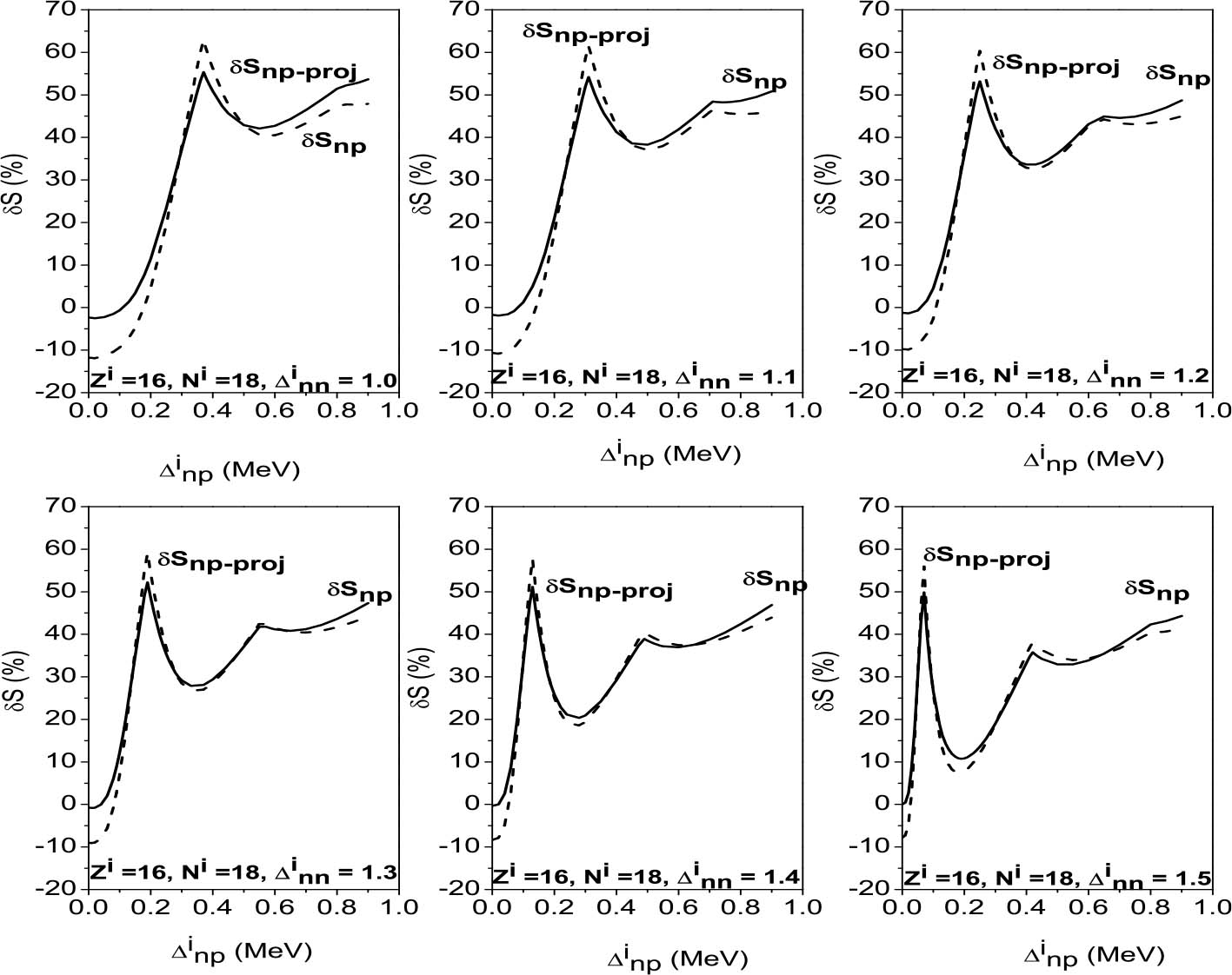
Fig. 2. Variations of the relative discrepancies of the spectroscopic factors (see the text for notations) corresponding to a two-neutron stripping reaction, in the case of the system Ni = 18, Zi = 16, as a function of the np gap parameter  of the initial state, for several values of the neutron gap parameter of the initial state
  . Solid lines show values obtained before the projection, and dashed lines show those obtained after the projection.
Download figure:
Standard imageFinally, the variations of δSnp and δSnp−proj have also been studied as a function of the np gap parameter of the final state  for given values of the other gap parameters. They are displayed in Fig. 3 in the case of a two-neutron stripping reaction for the system Ni = Zi = 16 with the parameters
  ,
,  MeV,
MeV,  and
and  . One observes important variations versus
  , as well as versus
  in these graphs. It thus appears that the np pairing effect strongly depends not only on the gap parameters of the initial state, but also on those of the final state. All these parameters thus have to be carefully chosen.

Fig. 3. Variations of the relative discrepancies of the spectroscopic factors corresponding to a two-neutron stripping reaction, in the case of the system Ni=Zi=16, as a function of the np gap parameter  of the final state, for several values of the neutron gap parameter of the initial state
  . Solid lines show values obtained before the projection, and dashed lines show those obtained after the projection.
Download figure:
Standard image3.1.2. Projection effect
In order to evaluate the projection effect, in the pairing between like particles, as well as in the np pairing case, let us define the relative discrepancies
and
We consider hereafter the same systems as in Figs. 1–3, with the same parameters. The variations of δSproj (in the case of pairing between like particles) and δSproj–np (in the np pairing case) which correspond to a two-neutron stripping reaction for the system Zi = Ni = 16 are displayed in Fig. 4 as a function of the np gap parameter of the initial state  for given values of the other gap parameters. In Fig. 5 are displayed the variations of the same quantities versus
  in the case of a two-neutron stripping reaction for the system Zi = 16, Ni = 18. Finally, Fig. 6 shows the variations of δSproj and δSproj–np as a function of the np gap parameter of the final state
  in the case of a two-neutron stripping reaction for the system Zi=Ni=16.

Fig. 4. Variations of the relative discrepancies of the spectroscopic factors (see the text for notations) corresponding to a two-neutron stripping reaction, in the case of the system Ni=Zi=16, as a function of the np gap parameter  of the initial state, for several values of the neutron gap parameter of the initial state
  . Solid lines show values obtained in the pairing between like particles, and dashed lines show values obtained in the np pairing case.
Download figure:
Standard image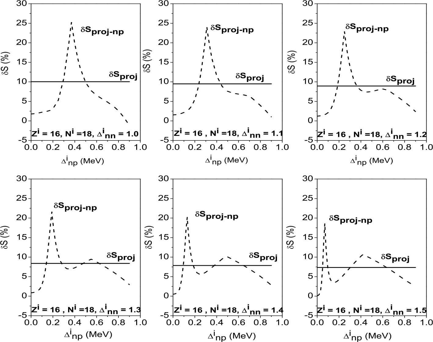
Fig. 5. Variations of the relative discrepancies of the spectroscopic factors (see the text for notations) corresponding to a two-neutron stripping reaction, in the case of the system Zi=16, Ni=18, as a function of the np gap parameter  of the initial state, for several values of the neutron gap parameter of the initial state
  . Solid lines show values obtained in the pairing between like particles, and dashed lines show values obtained in the np pairing case.
Download figure:
Standard image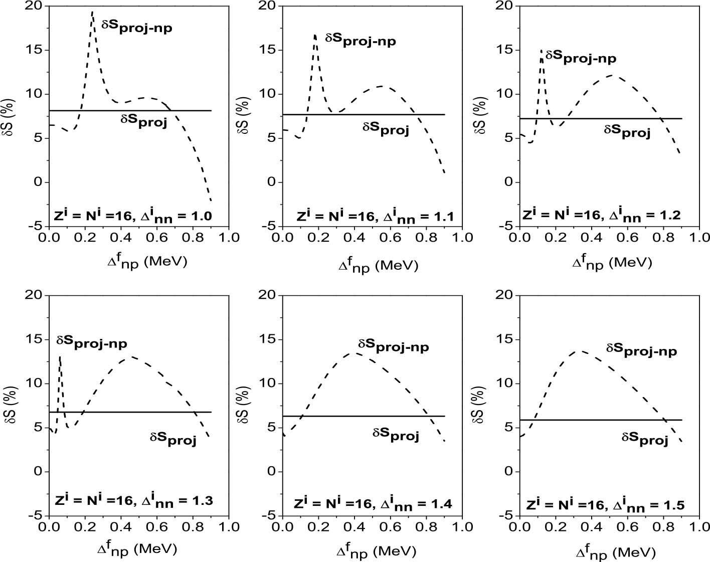
Fig. 6. Variations of the relative discrepancies of the spectroscopic factors corresponding to a two-neutron stripping reaction, in the case of the system Ni=Zi=16, as a function of the np gap parameter  of the final state, for several values of the neutron gap parameter of the initial state
  . Solid lines show the values obtained in the pairing between like particles, and dashed lines show the values for the np pairing case.
Download figure:
Standard imageIn each case, δSproj (i.e., in the pairing between like particles) is obviously constant as a function of  and has been represented only as a marker.
In the case Zi=Ni, it may be seen that all the curves in Fig. 4 behave similarly, as was the case for the np pairing effect. Moreover, one observes a maximum in the δSproj–np values at the same position as those in the δSnp and δSnp–proj curves (see Figs. 1 and 4, as well as Table 3). From Fig. 4, it may also be seen that the projection effect only corresponds to a decreasing of the SF values in the pairing between like particles. In the np pairing case, it may correspond either to an increasing or a decreasing of the SF values.
On the other hand, from Fig. 4, it appears that the projection effect seems to be more important in the np pairing case than in the pairing between like particles (see also Table 4, where the average values of δSproj and δSproj–np are reported). From Table 4, one may also conclude that the projection effect is less important that the np pairing effect. However, the particle-number fluctuation effect is non-negligible, since it may reach up to 35%.
In the case Zi ≠ Ni (Zi = 16, Ni = 18), comparing Fig. 2 and Fig. 5 enables one to see that the variations of δSproj–np are smoother than those of δSnp–proj and δSnp. Indeed, in some cases, the second maximum which appears in the δSproj–np curves is barely visible. However, the position of the maxima is the same with respect to the np pairing effect or the projection effect. One also notes that the particle-number fluctuations effect is clearly less important than the np pairing effect. However, it is far from negligible, since it can reach up to 25%.
Finally, a comparison of the variations of δSnp and δSnp–proj, on the one hand (see Fig. 3), and those of δSproj and δSproj–np, on the other hand (see Fig. 6), as a function of the np gap parameter of the final state  in the case of the system Zi=Ni=16, leads to the same conclusions with respect to the variations of the same quantities as a function of
  .
.
In summary, the particle-number fluctuation effect is important and varies significantly as a function of the various gap parameter values. The latter must then be rigorously chosen.
3.2. Even-even proton-rich nuclei
In order to study the case of even-even proton-rich nuclei, we used the single-particle energies of a deformed Woods-Saxon mean-field [106] with the parameters described in Ref. [107]. We used a maximal shell number Nmax=10, which corresponds to a total level degeneracy Ω=455.
The used ground-state deformation parameters are those of Refs. [108] and [109]. It was pointed out in Section 3.1 that the pairing gap parameter values have a great influence on the SF values and have to be carefully chosen. This is why, in the present work, they are deduced using Eqs. (8)–(10) from the "experimental" odd-even mass differences, that is [9],

where M(Z,N) is the experimental mass value given in the Atomic Mass Evaluation 2012 (AME 2012) [110].
We have also first checked the convergence of the projection method in a realistic case. The variation of the values of the SF corresponding to a two-neutron stripping reaction  given by Eq. (32), and that corresponding to a two-proton pick-up reaction
  thinspace given by Eq. (33), as a function of the extraction degrees of the false component m and m', are reported in Table 5 and Table 6 respectively, for the case of the nucleus 36Ar, chosen as an example. It may be seen from Tables 5 and 6 that the convergence is very rapid and is observed starting from m=6 and m'=4, and m=4 and m'=4, respectively, whereas Eq. (18) predicts m,m'>222 in each case. This confirms the efficiency and the rapidity of the projection method. Indeed, the computing time is of the order of 24 seconds in both cases, on an Intel Pentium IV 3.2 GHz processor.
Table 5.
Variation of the SF values  (%), corresponding to a two-neutron stripping reaction,as a function of the extraction degrees of the false components m and m', in the case of the nucleus 36Ar. The BCS value is
  .
.
| m | m' |

|
m | m' |

|
|---|---|---|---|---|---|
| 0 | 0 | 50.626 | 5 | 0 | 42.535 |
| 0 | 1 | 51.897 | 5 | 1 | 43.617 |
| 0 | 2 | 52.137 | 5 | 2 | 43.804 |
| 0 | 3 | 52.139 | 5 | 3 | 43.807 |
| 0 | 4 | 52.138 | 5 | 4 | 43.807 |
| 0 | 5 | 52.138 | 5 | 5 | 43.807 |
| 0 | 6 | 52.138 | 5 | 6 | 43.807 |
| 0 | 7 | 52.138 | 5 | 7 | 43.807 |
| 0 | 8 | 52.138 | 5 | 8 | 43.807 |
| 1 | 0 | 41.290 | 6 | 0 | 42.535 |
| 1 | 1 | 42.365 | 6 | 1 | 43.616 |
| 1 | 2 | 42.555 | 6 | 2 | 43.804 |
| 1 | 3 | 42.557 | 6 | 3 | 43.806 |
| 1 | 4 | 42.557 | 6 | 4 | 43.806 |
| 1 | 5 | 42.557 | 6 | 5 | 43.806 |
| 1 | 6 | 42.557 | 6 | 6 | 43.806 |
| 1 | 7 | 42.557 | 6 | 7 | 43.806 |
| 1 | 8 | 42.557 | 6 | 8 | 43.806 |
| 2 | 0 | 42.386 | 7 | 0 | 42.534 |
| 2 | 1 | 43.466 | 7 | 1 | 43.615 |
| 2 | 2 | 43.654 | 7 | 2 | 43.803 |
| 2 | 3 | 43.656 | 7 | 3 | 43.806 |
| 2 | 4 | 43.657 | 7 | 4 | 43.806 |
| 2 | 5 | 43.658 | 7 | 5 | 43.806 |
| 2 | 6 | 43.657 | 7 | 6 | 43.806 |
| 2 | 7 | 43.657 | 7 | 7 | 43.806 |
| 2 | 8 | 43.657 | 7 | 8 | 43.806 |
| 3 | 0 | 42.534 | 8 | 0 | 42.534 |
| 3 | 1 | 43.615 | 8 | 1 | 43.616 |
| 3 | 2 | 43.803 | 8 | 2 | 43.803 |
| 3 | 3 | 43.805 | 8 | 3 | 43.805 |
| 3 | 4 | 43.805 | 8 | 4 | 43.806 |
| 3 | 5 | 43.806 | 8 | 5 | 43.806 |
| 3 | 6 | 43.806 | 8 | 6 | 43.806 |
| 3 | 7 | 43.806 | 8 | 7 | 43.806 |
| 3 | 8 | 43.806 | 8 | 8 | 43.806 |
| 4 | 0 | 42.537 | 9 | 0 | 42.533 |
| 4 | 1 | 43.618 | 9 | 1 | 43.615 |
| 4 | 2 | 43.806 | 9 | 2 | 43.802 |
| 4 | 3 | 43.808 | 9 | 3 | 43.805 |
| 4 | 4 | 43.808 | 9 | 4 | 43.805 |
| 4 | 5 | 43.808 | 9 | 5 | 43.805 |
| 4 | 6 | 43.808 | 9 | 6 | 43.805 |
| 4 | 7 | 43.808 | 9 | 7 | 43.806 |
| 4 | 8 | 43.808 | 9 | 8 | 43.806 |
Table 6.
Variation of the SF values  (%), corresponding to a two-proton pick-up reaction, as a function of the extraction degrees of the false components m and m', in the case of the nucleus 36Ar. The BCS value is
  .
.
| m | m' |

|
m | m' |

|
|---|---|---|---|---|---|
| 0 | 0 | 70.102 | 5 | 0 | 82.496 |
| 0 | 1 | 66.702 | 5 | 1 | 78.595 |
| 0 | 2 | 66.500 | 5 | 2 | 78.341 |
| 0 | 3 | 66.500 | 5 | 3 | 78.342 |
| 0 | 4 | 66.500 | 5 | 4 | 78.342 |
| 0 | 5 | 66.500 | 5 | 5 | 78.342 |
| 0 | 6 | 66.500 | 5 | 6 | 78.342 |
| 0 | 7 | 66.500 | 5 | 7 | 78.343 |
| 0 | 8 | 66.500 | 5 | 8 | 78.343 |
| 1 | 0 | 76.827 | 6 | 0 | 82.496 |
| 1 | 1 | 73.247 | 6 | 1 | 78.595 |
| 1 | 2 | 73.023 | 6 | 2 | 78.342 |
| 1 | 3 | 73.024 | 6 | 3 | 78.342 |
| 1 | 4 | 73.024 | 6 | 4 | 78.342 |
| 1 | 5 | 73.024 | 6 | 5 | 78.342 |
| 1 | 6 | 73.024 | 6 | 6 | 78.342 |
| 1 | 7 | 73.024 | 6 | 7 | 78.342 |
| 1 | 8 | 73.024 | 6 | 8 | 78.342 |
| 2 | 0 | 82.110 | 7 | 0 | 82.496 |
| 2 | 1 | 78.234 | 7 | 1 | 78.595 |
| 2 | 2 | 77.983 | 7 | 2 | 78.342 |
| 2 | 3 | 77.983 | 7 | 3 | 78.342 |
| 2 | 4 | 77.984 | 7 | 4 | 78.342 |
| 2 | 5 | 77.984 | 7 | 5 | 78.342 |
| 2 | 6 | 77.984 | 7 | 6 | 78.342 |
| 2 | 7 | 77.984 | 7 | 7 | 78.342 |
| 2 | 8 | 77.984 | 7 | 8 | 78.342 |
| 3 | 0 | 82.484 | 8 | 0 | 82.496 |
| 3 | 1 | 78.584 | 8 | 1 | 78.595 |
| 3 | 2 | 78.331 | 8 | 2 | 78.342 |
| 3 | 3 | 78.331 | 8 | 3 | 78.342 |
| 3 | 4 | 78.332 | 8 | 4 | 78.342 |
| 3 | 5 | 78.332 | 8 | 5 | 78.342 |
| 3 | 6 | 78.332 | 8 | 6 | 78.342 |
| 3 | 7 | 78.332 | 8 | 7 | 78.342 |
| 3 | 8 | 78.332 | 8 | 8 | 78.342 |
| 4 | 0 | 82.495 | 9 | 0 | 82.496 |
| 4 | 1 | 78.594 | 9 | 1 | 78.595 |
| 4 | 2 | 78.341 | 9 | 2 | 78.342 |
| 4 | 3 | 78.341 | 9 | 3 | 78.342 |
| 4 | 4 | 78.342 | 9 | 4 | 78.342 |
| 4 | 5 | 78.342 | 9 | 5 | 78.342 |
| 4 | 6 | 78.342 | 9 | 6 | 78.342 |
| 4 | 7 | 78.342 | 9 | 7 | 78.342 |
| 4 | 8 | 78.342 | 9 | 8 | 78.342 |
In what follows, we will use the values m=m'=10 in order to ensure convergence.
As the np pairing correlations are supposed to be maximal in N ≃ Z nuclei, we considered nuclei such as Ni−Zi=0,2. We avoid the case Ni−Zi=4 since it leads, in some cases, to Nf−Zf=6, and thus to a situation where the np pairing is negligible. Only nuclei of which the  (t, t' = n,p) values are available (i.e. such as 16⩽Z⩽48) have been considered. The values of the SF corresponding to two-neutron stripping and two-proton pick-up reactions are reported in Table 7. These values have been obtained used four different approaches: the conventional BCS approach before and after projection, and the generalized (np) BCS approach before and after projection. The values used for the "experimental" gap parameters of the initial state
  (t, t' = n,p) are also given. In the following, the isovector np pairing and projection effects are studied separately.
Table 7. Values of the pairing gap parameters in the initial state (columns (2) to (4)), the SF corresponding to a two-neutron stripping reaction using the conventional BCS (column 5), SBCS (column 6), BCS-np (column 7) and SBCS-np (column 8) approaches, and the SF corresponding to a two-proton pick-up reaction using conventional BCS (column 9), SBCS (column 10), BCS-np (column 11) and SBCS-np (column 12) approaches.
| nucleus |
 /MeV /MeV |
 /MeV /MeV |
 /MeV /MeV |
two-neutron stripping | two-proton pick-up | ||||||
|---|---|---|---|---|---|---|---|---|---|---|---|
| SBCS | SSBCS | SBCS–np | SSBCS–np | SBCS | SSBCS | SBCS–np | SSBCS–np | ||||
| 32S | 2.141 | 2.196 | 1.049 | 88.139 | 77.080 | 62.574 | 54.715 | / | / | / | / |
| 34S | 1.562 | 1.818 | 0.244 | 131.800 | 97.026 | 123.906 | 86.982 | / | / | / | / |
| 36Ar | 2.266 | 2.313 | 1.372 | 107.305 | 76.935 | 57.858 | 43.806 | 134.472 | 121.151 | 70.431 | 78.343 |
| 38Ar | 1.441 | 2.100 | 0.250 | 98.790 | 107.820 | 129.455 | 133.514 | 68.325 | 57.985 | 61.710 | 56.452 |
| 42Ca | 2.110 | 1.676 | 0.524 | 108.855 | 102.335 | 151.527 | 161.877 | 132.475 | 96.695 | 125.457 | 93.996 |
| 46Ti | 2.093 | 1.878 | 0.898 | 100.724 | 82.210 | 87.968 | 118.657 | 147.263 | 153.219 | 110.679 | 97.737 |
| 48Cr | 2.122 | 2.136 | 1.429 | 93.654 | 76.377 | 35.905 | 35.776 | 172.030 | 166.388 | 87.882 | 129.685 |
| 50Cr | 1.697 | 1.584 | 0.526 | 115.527 | 110.265 | 103.508 | 114.667 | 116.091 | 108.153 | 65.929 | 44.654 |
| 52Fe | 1.984 | 2.018 | 1.140 | 106.021 | 100.057 | 60.116 | 88.350 | 163.784 | 147.257 | 101.265 | 106.635 |
| 54Fe | 1.497 | 1.594 | 0.259 | 108.794 | 105.047 | 109.430 | 137.899 | 101.720 | 80.021 | 81.291 | 64.406 |
| 56Ni | 2.080 | 2.152 | 1.017 | 87.518 | 85.184 | 55.578 | 60.604 | 171.638 | 166.283 | 102.778 | 113.882 |
| 58Ni | 1.667 | 1.349 | 0.232 | 132.449 | 129.251 | 134.209 | 173.271 | 133.932 | 125.502 | 109.967 | 93.338 |
| 60Zn | 1.650 | 1.782 | 1.091 | 136.022 | 128.270 | 78.980 | 87.350 | 123.741 | 123.699 | 48.714 | 66.419 |
| 62Zn | 1.459 | 1.617 | 0.609 | 161.251 | 151.171 | 128.537 | 175.355 | 99.728 | 99.040 | 63.507 | 52.508 |
| 66Ge | 1.607 | 1.799 | 0.786 | 140.850 | 132.892 | 92.239 | 118.423 | 128.401 | 126.678 | 114.848 | 131.551 |
| 68Se | 2.112 | 2.047 | 1.529 | 117.307 | 104.343 | 21.078 | 45.908 | 202.582 | 203.016 | 50.726 | 92.018 |
| 70Se | 1.755 | 1.914 | 0.764 | 220.778 | 212.981 | 180.497 | 278.442 | 150.336 | 146.931 | 123.943 | 134.604 |
| 72Kr | 2.008 | 1.926 | 1.340 | 137.308 | 129.398 | 48.091 | 66.100 | 233.193 | 225.330 | 88.016 | 157.774 |
| 74Kr | 1.580 | 1.681 | 0.649 | 157.029 | 149.274 | 74.456 | 95.149 | 144.971 | 136.466 | 48.491 | 23.751 |
| 76Sr | 1.641 | 1.475 | 0.918 | 121.134 | 116.867 | 38.843 | 82.306 | 137.573 | 133.063 | 77.981 | 80.925 |
| 78Sr | 1.353 | 1.310 | 0.212 | 84.957 | 78.312 | 25.531 | 42.472 | 125.852 | 125.014 | 78.258 | 34.689 |
| 82Zr | 1.498 | 1.671 | 0.336 | 187.531 | 170.004 | 205.330 | 240.476 | 169.433 | 148.511 | 96.695 | 64.360 |
| 86Mo | 1.825 | 1.784 | 0.711 | 175.823 | 153.444 | 166.399 | 180.039 | 245.170 | 226.898 | 177.970 | 159.022 |
| 90Ru | 1.537 | 1.577 | 0.456 | 147.347 | 121.222 | 165.991 | 191.780 | 188.358 | 168.513 | 174.117 | 160.411 |
| 94Pd | 1.506 | 1.430 | 0.452 | 198.876 | 190.931 | 175.914 | 182.419 | 181.878 | 158.135 | 131.523 | 105.527 |
| 98Cd | 1.310 | 1.756 | 0.290 | 130.510 | 127.857 | 124.096 | 145.897 | 143.745 | 112.870 | 136.813 | 113.803 |
3.2.1. Neutron-proton pairing effect
The np pairing effect, both before and after the projection, has been studied by means of the relative discrepancies δSnp and δSnp–proj defined by Eqs. (41) and (42). The variations of these quantities as a function of the atomic number of the initial state Zi are reported in the left-hand part of Fig. 7 and Fig. 8 for two-neutron stripping and two-proton pick-up reactions respectively, for (Ni−Zi) = 0,2. For both kinds of reaction, there are significant variations in the δSnp and δSnp–proj values from one nucleus to another. Moreover, the δSnp and δSnp–proj values may be very important, as was already the case within the Richardson model, and may reach up to 80% in absolute value.
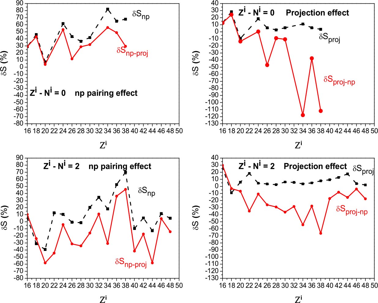
Fig. 7. (color online) np pairing effect (left) and projection effect (right) on the spectroscopic factors, in the case of a two-neutron stripping reaction, as a function of Zi for (Ni−Zi) = 0,2. See the text for notations.
Download figure:
Standard image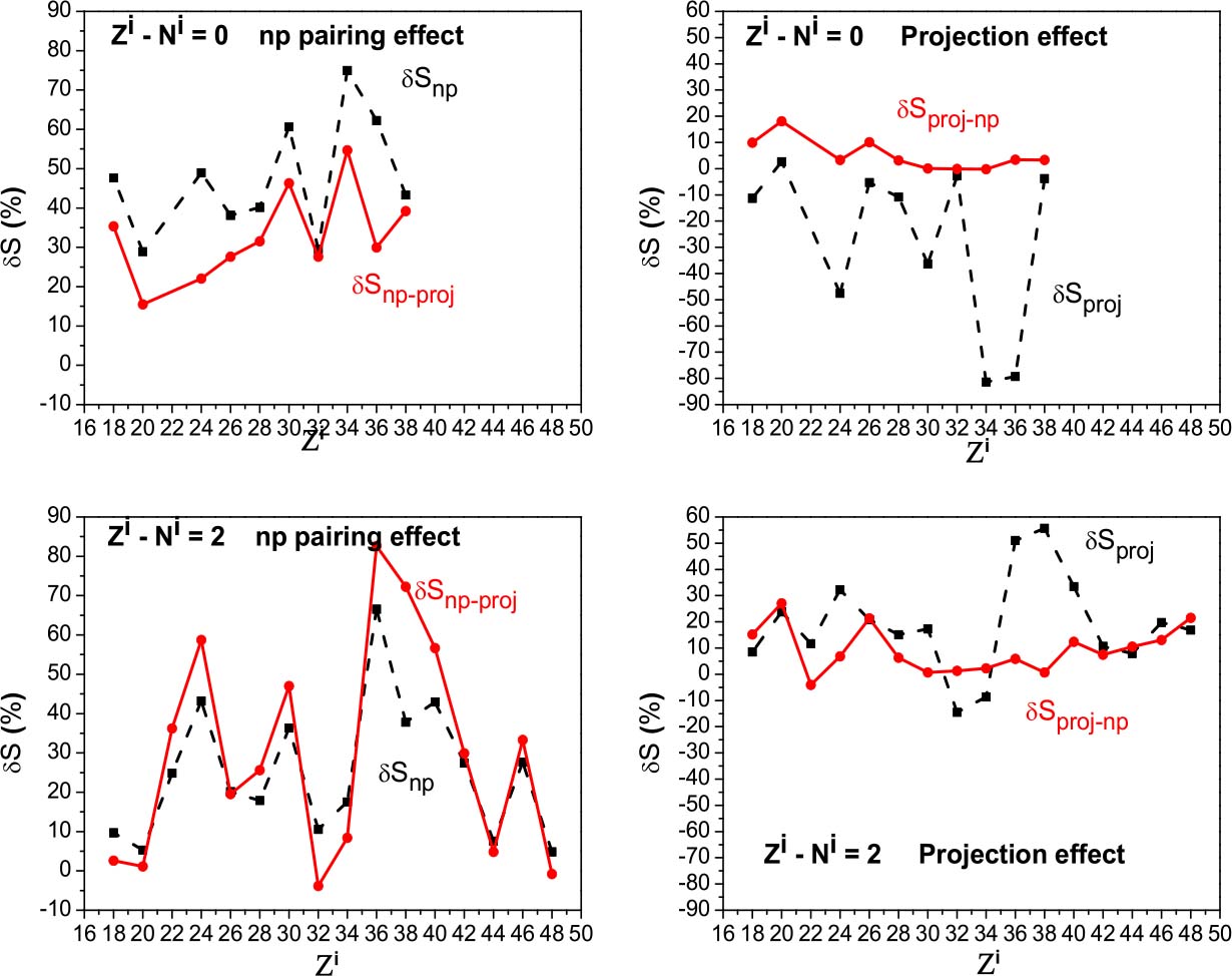
Fig. 8. (color online) np pairing effect (left) and projection effect (right) on the spectroscopic factors, in the case of a two-proton pick-up reaction, as a function of Zi for (Ni−Zi) = 0,2. See the text for notations.
Download figure:
Standard imageMoreover, the np pairing effect seems to be of the same order of magnitude in the two-neutron stripping and the two-proton pick-up reactions.
One may also observe that, when Ni=Zi, the np pairing effect only results in a decrease of the SF values. By contrast, when (Ni−Zi)=2, this effect can be reflected either in an increase or a decrease of the SF values.
Figures 7 and 8 show a decrease, on average, of the absolute value of δSnp and δSnp–proj as a function of (Ni−Zi). The average absolute values of these quantities are reported in Table 8 as a function of (Ni−Zi). It is worth noticing that, even if the overall values of  and
and  are close to each other, the decrease of
  as a function of (Ni−Zi) is less clear after the projection than before it, for both kinds of reaction.
Table 8.
Variations of the average absolute values of the discrepancies δS as a function of Ni−Zi. The  values are given in %.
| two-neutron stripping | ||||
| Ni−Zi |

|

|
|δSproj| | |δSproj–np| |
| 0 | 48.08 | 33.60 | 10.30 | 38.45 |
| 2 | 20.04 | 28.30 | 8.49 | 24.46 |
| total | 30.43 | 30.27 | 9.16 | 29.64 |
| two-proton pick-up | ||||
| Ni−Zi |

|

|
|δSproj| | |δSproj–np| |
| 0 | 47.44 | 32.97 | 5.14 | 28.10 |
| 2 | 25.01 | 29.62 | 9.26 | 18.84 |
| total | 33.63 | 31.27 | 7.99 | 24.18 |
The fact that the np pairing effect on the SF diminishes as a function of (Ni−Zi) was foreseeable, since it is now well established that Δnp is maximal when N=Z and decreases as a function of (N–Z) [7].
3.2.2. Projection effect
The projection effect, in the case of pairing between like particles as well as in the case of isovector pairing, has been studied using the relative discrepancies δSproj and δSproj–np defined by Eqs. (43) and (44). Their variations as a function of the atomic number of the initial state Zi are reported in the right-hand part of Fig. 7 and Fig. 8 in the case of two-neutron stripping and two-proton pick-up reactions respectively, for (Ni−Zi)=0,2. From Figs. 7 and 8, one may observe fluctuations of δSproj and δSproj–np which may be sometimes important. However, these fluctuations are less pronounced in the pairing between like particles than in the isovector pairing case, in which they may reach up to 120% in absolute value. The projection effect is thus not systematic and varies from one nucleus to another.
It may also be seen that the particle-number projection effect can be reflected both by an increase and a decrease of the SF values.
It also appears that the particle-number fluctuation effect is, on average, much more important in the np pairing case than in the pairing between like particles. This fact is more visible in Table 8 where we report the average values of |δSproj|, and |δSproj–np|. These results confirm those obtained within the Richardson model.
Moreover, from Figs. 7 and 8, one may also conclude that the particle-number fluctuation effect is overall lower than the np pairing effect. This has already been observed in the schematic case.
As a conclusion, the effects of isovector pairing and particle-number projection on the SF values for these kinds of reactions in proton-rich nuclei are far from negligible and must be taken into account.
4. Conclusion
Isovector np pairing and particle-number fluctuation effects on the SF corresponding to one-pair like-particle transfer reactions in proton-rich even-even nuclei have been studied. Using a schematic definition proposed by Chasman [104], expressions of the SF corresponding to two-neutron stripping and two-proton pick-up reactions, which take into account the isovector np pairing effect, have been established within the generalized BCS approach. Expressions of the same SF have been also established within the discrete SBCS particle-number projection method. In both cases, it is shown that these expressions generalize those obtained in the pairing between like-particles case. As a first step, the formalism has been tested using the schematic Richardson model. It has thus been shown that the inclusion of the isovector pairing correlations is necessary when calculating the SF of these kinds of reactions. It is also necessary to perform a particle-number projection. Finally, one has to carefully choose the pairing-strength values, either in the initial or the final state.
As a second step, we used the single-particle energies of the Woods-Saxon deformed mean field.
Since the np pairing correlations affect only systems such as N close to Z, we considered nuclei such as (N – Z) = 0,2. Only nuclei of which the "experimental" values of the pairing gap parameters Δpp, Δnn and Δnp are known were taken into consideration. In this way, the pairing-strength values Gpp, Gnn and Gnp are directly deduced.
It was shown that the isovector np pairing effect on the SF values, either before or after the projection, is important since the relative discrepancies with the pairing between like-particle calculations may reach up to 80%. It was also shown that this effect diminishes as a function of (N – Z).
The particle-number fluctuation effect appears to be less important, on average, than the np pairing effect. It is, however, far from negligible. It also appears that there is no systematics in the projection effect, which may vary from one nucleus to another.
Appendix A: Pairing between like particles
Appendix. Wave functions
In the pairing between like particles, the BCS ground-state of a system constituted by (2Pt), t=n,p, paired particles (neutrons or protons) is given by [29]
ujt and vjt are the inoccupation and occupation probability amplitudes of the single-particle state |jt⟩ of energy εjt, created by the operator  . They are given by
 being the half-width of the gap and λt the energy of the Fermi-level.
After projection, the SBCS ground-state is given by [51]

where ξk and zk are defined by Eq. (14), m is a non-zero integer so called extraction degree of the false components, cc means the complex conjugate with respect to zk and
The normalization constant Cmt is given by
Let us note that the following property

which is satisfied by any operator  which conserves the particle number, has been used in the derivation of Eq. (5).
As soon as

the state |ψm⟩t converges towards the state with the good particle-number. In Eq. (A6), Ωt is the total degeneracy of states.
Appendix. Spectroscopic factors
The wave function which describes the nucleus in its initial (or final) state is defined in the pairing between like particles as the product of the two wave functions which correspond to the neutron and proton systems. In what follows, the calculation of the SF will be performed by assuming that the neutron (or proton) system is not affected by the proton (or neutron) transfer.
Before projection
In this case, the total wave function is given by

where |BCS⟩t (t=n,p) is given by Eq. (A1). The SF in the case of the transfer of one pair of paired like-particles, defined by Eq. (19) and Eq. (20), then become
After projection
In this case, the total wave function is given by
Using the property (17), one has


where the fact that  has been taken into account.
It has been assumed here that the convergence is reached for the same value m of the extraction degrees of the false components of the wave function of the initial and final states.
Let us also note that the use of the property (17) has led to expressions easier to handle than those obtained in Ref. [103].