
Abstract
We study a forced variable-coefficient extended Korteweg–de Vries (KdV) equation in fluid dynamics with respect to internal solitary wave. Bäcklund transformations of the forced variable-coefficient extended KdV equation are demonstrated with the help of truncated Painlevé expansion. When the variable coefficients are time-periodic, the wave function evolves periodically over time. Symmetry calculation shows that the forced variable-coefficient extended KdV equation is invariant under the Galilean transformations and the scaling transformations. One-parameter group transformations and one-parameter subgroup invariant solutions are presented. Cnoidal wave solutions and solitary wave solutions of the forced variable-coefficient extended KdV equation are obtained by means of function expansion method. The consistent Riccati expansion (CRE) solvability of the forced variable-coefficient extended KdV equation is proved by means of CRE. Interaction phenomenon between cnoidal waves and solitary waves can be observed. Besides, the interaction waveform changes with the parameters. When the variable parameters are functions of time, the interaction waveform will be not regular and smooth.
Export citation and abstract BibTeX RIS
1. Introduction
The internal solitary waves are nonlinear waves propagating in a shallow and stratified layer. They are frequently observed close to the oceanic regions of steep topography such as shelf-edges, ridges, and sills.[1–3] Internal solitary waves in the shallow water can be described by the Korteweg–de Vries (KdV) equation.[4–6] The KdV equation can also describe some wave phenomena in the atmosphere, plasma, astrophysics, and transmission lines.[7,8]
With the increasing observations on internal solitary waves, more and more factors are added to generalize this model, such as variable depth, cubic nonlinear term, Coriolis effect, horizontal variability of the density, and shear flow stratification. Given these considerations, the extended KdV equation has been introduced, which contains both the quadratic and cubic nonlinearities. The extended KdV equation can well describe the solitary waves that observed in a laboratory experiment if the nonlinear terms are smaller compared with the linear wave speed. In the marine and geophysical applications, it is necessary to consider an external force when the waves are generated by the moving ships or flows over the bottom topography.[9] In this paper, we will focus on the forced variable-coefficient extended KdV equation in the form of Ref. [9]
here the variable coefficients α1(t), α2(t), α3(t), α4(t), α5(t), and Γ (t) are smooth functions of t, variables x and t are the scaled space and time coordinates, Γ (t) is the external time-dependent force, and u is the wave function determining the time evolution of the vertical displacement on the isopycnal surface. The equation can describe the weakly nonlinear long internal solitary waves in the fluid with continuous stratification on the density if the external force term Γ(t) vanishes. By means of the Hirota bilinear method, multi-soliton solutions of the forced variable-coefficient extended KdV equation (1) have been derived in Ref. [9]. The effects of the external time-dependent force and the inhomogeneities were have been discussed.[9] The Painlevé integrability of Eq. (1) was tested by virtue of Painlevé analysis in Ref. [10]. By means of the truncated Painlevé expansion, an analytic solution of Eq. (1) was proposed.[10]
With respect to the internal solitary wave dynamics about several oceanic shelves, when α1(t) = β1, α2(t) = β2, α3 (t) = β3, α4 (t) = β4, α5 (t) = 0, and Γ (t) = 0, equation (1) reduces to the following extended equation:

where the coefficients β4, β3, β1, and β2 are the wave speed, dispersion parameter, quadratic, and cubic nonlinear coefficients, respectively.[11] Numerical simulation of Eq. (2) is carried out to interpret that an internal solitary waves may maintain its soliton-like form for the large distances, which confirms why internal solitary waves are widely observed in oceans.[11] In the investigation on the internal waves in a stratified ocean when the pycnocline lies midway between the sea bed and surface, the model[12] is researched in the form of

with α1(t) = β5(t), α2(t) = β6, α3(t) = 1, α4 (t) = 0, α5(t) = 0, Γ (t) = 0, where the variable coefficient β(t) and parameter ν denote the quadratic and cubic nonlinear coefficients, respectively. The authors in Ref. [12] researched the solitary wave transformation in a zone. When α2(t) = 0, equation (1) reduces to the forced variable-coefficient KdV equation in the form of

which can be applied in the internal solitray wave dynamics, but also can be used to describe the propagation of the weakly nonlinear waves in a composite medium.[13]
Many effective methods have been proposed to analyze partial differential equations, such as Painlevé analysis,[14–16] symmetry group,[17–19] consistent Riccati expansion (CRE),[20–22] and so on.[23,24] To our knowledge, the CRE solvability, symmetries and cnoidal-solitary wave interaction solutions of the forced variable-coefficient extended KdV equation have not been studied. Although the truncated Painlevé analysis of Eq. (1) has been studied in Ref. [10], more results can be obtained by means of the truncated Painlevé expansion. The main aim of this paper is to research Bäcklund transformations, CRE solvability, symmetries, and interaction solutions of the forced variable-coefficient extended KdV equation (1). The outline of the paper is as follows. In Section 2, truncated Painlevé expansion is applied to Eq. (1), some Bäcklund transformations of Eq. (1) are obtained, and some solitary wave solutions by means of truncated Painlevé expansion are demonstrated. Section 3 is devoted to symmetries and one-parameter group transformations of Eq. (1). In Section 4, with the help of function expantion method, cnoidal wave solutions and solitary wave solutions of Eq. (1) with some parameter constraints are proposed. The CRE solvability of Eq. (1) is proved in Section 5. In Section 6, cnoidal-solitary wave interaction solutions of Eq. (1) are discussed by means of CRE method. The final section concludes our conclusion and discussion.
2. Truncated Painlevé expansion and Bäcklund transformations of the forced variable-coefficient extended KdV equation
The Painlevé analysis method is an efficient analytic method to solve nonlinear partial differential equations.[25–27] In this section, we will use the truncated Painlevé expansion to analyze the forced variable-coefficient extended KdV equation. Truncated Painlevé expansion of the forced variable-coefficient extended KdV equation (1) can be written as
where u0, u1, and f are functions of {x,t}, and f is the singular manifold function. Substituting Eq. (5) into Eq. (1), and collecting different coefficients of f, and setting these coefficients to be zeros, one can obtain the formulas of {u0,u1} and the parameter constraints. From the coefficient of f−4, we obtain
where δ1 = ± 1. The coefficient of f−3 concludes that
The substitution of Eqs. (6) and (7) into the coefficient of f−2 leads to
or
where
S and C are invariant for the Möbious transformation
When
equation (8) will degenerate to
where C1 and C2 are arbitrary constants. Equation (13) is the Schwarzian form of Eq. (1) with parameter constraint Eq. (11). Substituting Eqs. (6)–(8) into Eq. (1) yields
From the above calculations, we can derive the following two theorems.
Theorem 1 (Bäcklund transformation theorem) If f satisfies Eq. (8), then
is a solution of the forced variable-coefficient extended KdV, with the parameters satisfying Eq. (14).
Theorem 2 (Bäcklund transformation theorem) If f satisfies Eq. (8), then
is a solution of the forced variable-coefficient extended KdV equation (1), where the parameters satisfying Eq. (14).
One can obtain analytic solutions of a researched system from a truncated Painlevé expansion. For f, we introduce the ansatz
where f should satisfy the relationship Eq. (8). Substituting formula Eq. (17) into Eq. (8) yields
where C3 is an integral constant.
Using Eqs. (17) and (18) into Eq. (16) gives the solitary wave solution
where the parameters satisfying Eq. (14), and a and b are arbitrary constants. The evolution of u with x and t is demonstrated in Fig. 1, where the parameters are given by
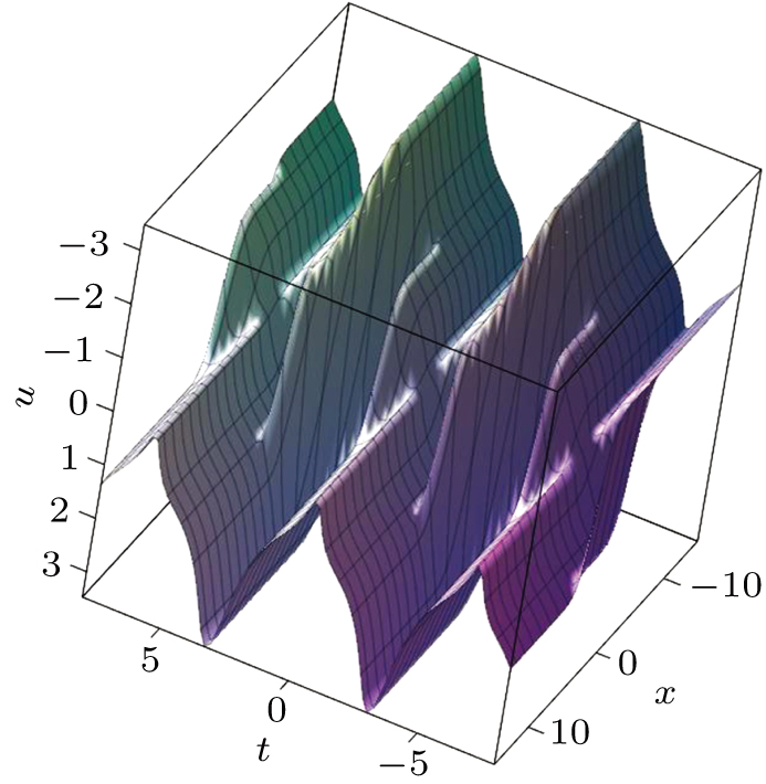
Fig. 1. The evolution of u with x and t, with the parameters given in Eq. (20).
Download figure:
Standard imageFigure 1 shows that u is a dark solitary wave at one fixed time, while it evolves periodically over time, because the parameters are time-periodic.
3. Symmetries of the forced variable-coefficient extended KdV equation
Symmetry theory is one powerful method for researching partial differential equations.[18,19,28,29] For the forced variable-coefficient extended KdV equation (1), the symmetry determining equation can be written as
where σ is the symmetry of u in the forced variable-coefficient extended KdV equation, and it is a function of x and t. σ can be supposed to have the form

where X (x,t,u), T (x,t,u), and U (x,t,u) are functions of {x,t,u}. Formula (22) implies that equation (1) is formal invariant under the transformation

where  is an infinitesimal parameter. Substituting Eq. (22) into Eq. (21), and simplifying some terms by the original equations, we obtain an over-determined set of equations for the unknown functions { X, T, U }. Solving the determinant equations, we can obtain the solutions of { X, T, U }.
The variable coefficients α1(t), α2(t), α3(t), α4(t), and Γ (t) in Eq. (1) break the symmetries on time, and the term of α5(t) u breaks the symmetry of translation invariance on u. If the parameters are completely free and unrestricted, the symmetry σ is very simple, which is in the form of

with λ being a constant. Thus, the symmetry vector is ∂/∂x , which means translation invariance on space x. We introduce the parameter constant Eq. (14), then the symmetry σ of Eq. (1) is increased, and X(x,t,u), T (x,t,u), and U (x,t,u) are in the form of

where F(t) in Eq. (25b) is determined by
A general element of the symmetry algebra is described as
The invariant group vectors can be written as

where
where V1 and V2 mean scaling transformations, and V3 is related to Galilean boosts. The terms of ∂/∂ t in V1 and V2 shows that time t is a changing variable, which means the parameters on α1(t), α2(t), α3(t), α5(t), and Γ(t) are functions of changing variable t. In this case, to obtain some one-parameter invariant subgroups from the vectors are very complicated.
If the concrete forms of α1(t), α2(t), α3(t), α5(t), and Γ(t) are determined, to obtain some one-parameter invariant subgroups from the V1 and V2 is still possible. For example, we consider the ansatz

then, V1 is simplified to be
The corresponding one-parameter invariant subgroup is
By means of one-parameter subgroups, one can obtain the corresponding subgroup invariant solutions. If u(x,t) is an analytic solution of the forced variable-coefficient extended KdV equation (1), then so is the function
For another example, we introduce the ansatz

Thus, V2 can be rewritten as
then, we can obtain the one-parameter invariant subgroup in the form of
with
This gives the subgroup invariant solution in turn
Because there is no ∂/∂ t in V3(F(t)), it is easy to obtain the one-parameter invariant subgroup from V3(F(t)), which is in the form of

Then, we obtain the subgroup invariant solutions. If {u(x,t)} is an analytic solution of the forced variable-coefficient extended KdV equation (1), then so is the function

4. Cnoidal wave solutions and solitary wave solutions of the forced variable-coefficient extended KdV equation
As far as the travelling wave solutions are concerned, one can always use the transformtions

where ω1 and k1 are real numbers and ω1/k1 means the speed of the propagating waves. Equation (1) is thus transformed to a nonlinear ordinary differential equation as
For a general consideration of cnoidal wave solutions, we consider the ansatz

where d0, d1, d2, and m1 are real numbers, which are undetermined parameters. Substituting Eq. (43) into Eq. (42), and setting all coefficients of sn(ξ,m1), cn(ξ,m1), and dn(ξ,m1) to zeros, one can determine the parameters. These coefficients imply that α5(t) and Γ (t) should be zero, otherwise, there is no effective cnoidal wave solution. When α5(t) = Γ (t) = 0, there are the following two nontrivial solutions to the forced variable-coefficient extended KdV equation.
(i) Cnoidal wave solution 1:

where α2 (t) α3 (t) > 0, and α1 (t), α2 (t), and α3 (t) are linear to each other.
(ii) Cnoidal wave solution 2:

where α2 (t) α3 (t) < 0, and α1 (t), α2 (t), and α3 (t) are linear to each other. If m1 = 1, the cnoidal wave solutions will reduce back to soliton solutions. The cnoidal wave solution 1 becomes a bright soliton solution

The cnoidal wave solution 2 turns to a dark soliton solution

5. CRE solvability of the forced variable-coefficient extended KdV equation
We will analyze the forced variable-coefficient extended KdV equation by means of the CRE method[20–22] in this section. The Riccati equation is written in the following form:

where a0, a1, and a2 are arbitrary constants. For the Riccati equation, there is the solution in the form of
with

For a system
one can assume that it can be expanded as
where T(w) is an analytic solution of the Riccati equation. Substituting Eq. (52) into Eq. (51), and letting all the coefficients of Ti (w) to be zeors, one will obtain a conditional system

If the system Eq. (53) is consistent, then the expansion Eq. (52) is a 'CRE' and the nonlinear system Eq. (51) is 'CRE'-solvable.[22]
In order to obtain cnoidal-solitary wave interaction solutions, one will apply CRE method to analyze Eq. (1). The CRE method is proposed to identify CRE-solvable systems and look for interaction solutions between solitons and cnoidal waves of nonlinear excitations. For the forced variable-coefficient extended KdV equation, u can be expanded as the truncated expansion in the form of

where u2, u3, and w are all functions of x and t, and T(w) is a solution of the Riccati equation.
Substituting Eqs. (48) and (54) into Eq. (1), and letting all coefficients of different powers on T(w) to be zeros, we find that
where the parameters are constrained by Eq. (14), and w is governed by
According to the definition CRE and CRE-solvable, the forced variable-coefficient extended KdV equation is obviously CRE-solvable. Based on the above discussion, we have the following theorem.
Theorem 3 (CRE solvability theorem)
The forced variable-coefficient extended KdV equation is a CRE solvability system. If w is a solution of the consistent condition Eq. (56), then u in the form of
is a solution of the forced variable-coefficient extended KdV equation, where the parameters, T(w) and θ are given by Eqs. (14), (49), and (50), respectively.
6. Cnoidal-solitary wave interaction solutions of the forced variable-coefficient extended KdV equation
From the CRE of the Boussinesq equation, we can further research analytic solutions of the Boussinesq equation. The substitution of Eq. (49) into Eq. (57) leads to
Formula (58) shows that if we want to know the concrete form of u, the expression of w is needed. To determine the cnoidal-solitary wave interaction solutions, we introduce the ansatz

where k2, k3, ω2, ω3, a3, n, and ν are constants, and Eπ is the third type of incomplete elliptic integral. Plugging Eq. (59) into Eq. (58) yields
where
Substituting Eq. (59) into Eq. (56), and letting all coefficients of different powers of sn(k3 x + ω3 t, ν) be zeros, we find that the parameters should satisfy the relationships in the form of
The evolution of u with parameters Eq. (63) is depicted in Fig. 2. The concrete forms of the parameters are as follows:
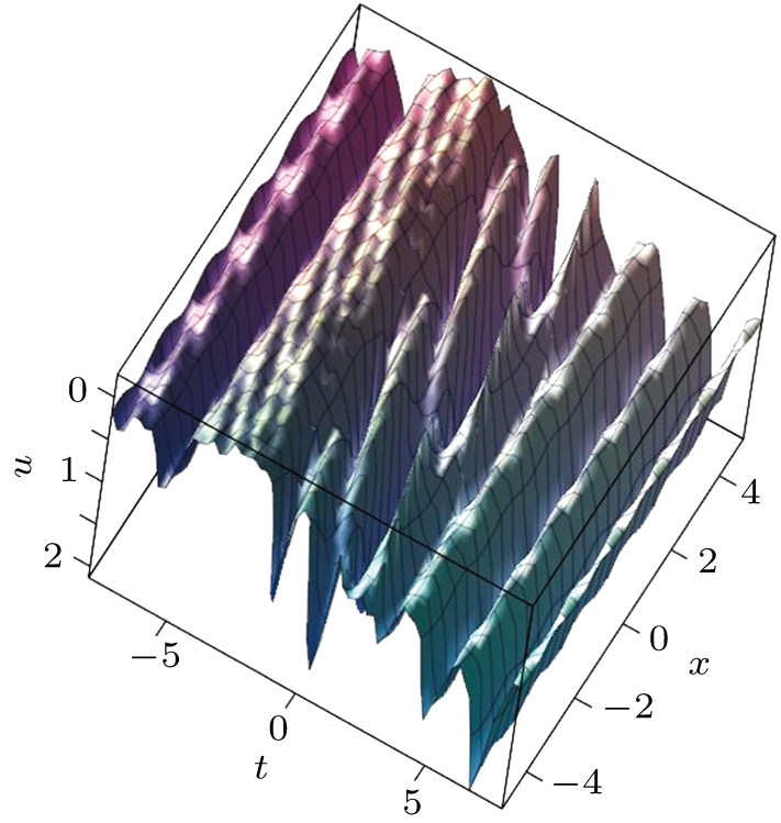
Fig. 2. Interaction wave solutions of u between cnoidal waves and bright waves, where the parameters are given in Eq. (67).
Download figure:
Standard imageEvolutions of u in Fig. 2 are interaction waves between bright waves and cnoidal waves. Because the parameters are functions of time, the evolution curve is not very regular and smooth.
The solution of u in Eq. (60) with parameter relationships Eq. (66) is proposed in Fig. 3. The concrete forms of the parameters are as follows:
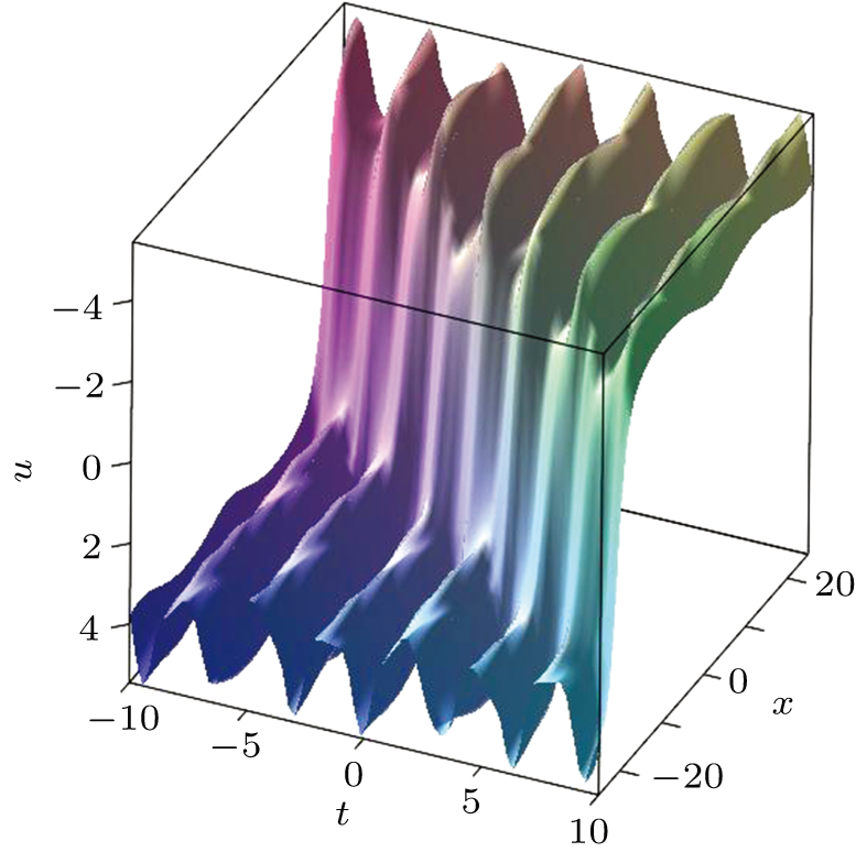
Fig. 3. Interaction wave solution of u between cnoidal waves and dark waves, where the parameters are given in Eq. (68).
Download figure:
Standard imageFigure 3 displays the interaction behavior between dark solitary waves and cnoidal waves, where cnoidal waves reside on dark solitary waves.
7. Summary and discussion
In this paper, a forced variable-coefficient extended KdV equation in fluid dynamics of internal solitary waves was researched. Truncated Painlevé expansion for Eq. (1) is carried out. Bäcklund transformations of the forced variable-coefficient extended KdV equation are demonstrated. A solitary wave solution is proposed by means of truncated Painlevé expansion. When the parameters {αi (t),i = 1,2,3,4,5} and the external time dependent force Γ(t) are assumed to be trigonometric periodic functions, the wave function is a dark solitary wave at one fixed time, which it evolves periodically over time.
Symmetry calculation on forced variable-coefficient extended KdV equation shows it is invariant under the Galilean transformations and the scaling transformations. One-parameter group transformations and one-parameter subgroup invariant solutions are presented. Cnoidal wave solutions and solitary wave solutions of Eq. (1) are obtained by means of function expansion method. CRE method is applied to study the forced variable-coefficient extended KdV equation, and the CRE solvability of the model is proved by CRE. Interaction phenomenon between cnoidal waves and solitary waves can be observed. The interaction waveform changes with the parameters. When the parameters are functions of time, the evolution curve will be not regular and smooth. Another interaction mode between solitons and other nonlinear excitations is soliton molecule, which is first discovered in optical systems. The resonance condition of soliton molecules is velocity resonance, and it is a new resonance condition. Now, soliton molecules have been found in fluid, Bose–Einstein condensates, particle physics, and so on. The resonance of the forced variable-coefficient extended KdV equation is an open problem.
The above analytic methods and results could be expected to helpfully understand the fluid dynamics of internal solitary waves. The famous KdV equation has wide applications in many fields, such as atmosphere, plasma, astrophysics, and transmission lines. As a forced variable-coefficient extended KdV equation, the application of Eq. (1) should be not only in the field of internal solitary waves, but also in more fields. These applications of the forced variable-coefficient extended KdV equation need further study.
Acknowledgement
The authors would like to thank Professor Sen-Yue Lou for his valuable discussion.
Footnotes
- *
Project supported by the National Natural Science Foundation of China (Grant Nos. 11775047, 11775146, and 11865013).