

Abstract
In this paper, a new approach is devoted to find novel analytical and approximate solutions to the damped quadratic nonlinear Helmholtz equation (HE) in terms of the Weiersrtrass elliptic function. The exact solution for undamped HE (integrable case) and approximate/semi-analytical solution to the damped HE (non-integrable case) are given for any arbitrary initial conditions. As a special case, the necessary and sufficient condition for the integrability of the damped HE using an elementary approach is reported. In general, a new ansatz is suggested to find a semi-analytical solution to the non-integrable case in the form of Weierstrass elliptic function. In addition, the relation between the Weierstrass and Jacobian elliptic functions solutions to the integrable case will be derived in details. Also, we will make a comparison between the semi-analytical solution and the approximate numerical solutions via using Runge–Kutta fourth-order method, finite difference method, and homotopy perturbation method for the first-two approximations. Furthermore, the maximum distance errors between the approximate/semi-analytical solution and the approximate numerical solutions will be estimated. As real applications, the obtained solutions will be devoted to describe the characteristics behavior of the oscillations in RLC series circuits and in various plasma models such as electronegative complex plasma model.
Export citation and abstract BibTeX RIS
1. Introduction
The Helmholtz equation (HE) or sometimes called reduced wave equation is a second-order differential equation (DE) which it is used in a lot in physics and mathematics to explain many phenomena. One of the most important mathematical formulas for linear HE is given by:  where ∇2, k, and Φ represent the Laplace operator, wavenumber, and the amplitude of oscillation, respectively. This equation is related to many applications in physics problem-solving concepts like seismology, acoustics and electromagnetic radiation, acoustic waves in plasma physics, ocean, also in optical fibers [1–6]. For instance, Liu and Holt [6] used the HE solutions for studying and investigating wave gradiometry and its application to USArray in the eastern U.S. Lin and Ritzwoller [7] used the solutions of HE for improving surface wave tomography. Also, the HE is related to the acoustic-wave equation:
  , where cs and
  are, respectively, the acoustic speed and acoustic pressure. By inserting
  into the acoustic-wave equation, we can get the HE:
  , where
 ![${k}^{2}=-\left[1/{c}_{{\rm{s}}}^{2}T\left(t\right)\right]{\partial }_{t}^{2}T\left(t\right)$](https://content.cld.iop.org/journals/0253-6102/73/3/035501/revision3/ctpabda1bieqn6.gif) .
.
It is known that the HE has different formulas and these formulas have been solved analytically and numerically using several approaches and techniques. For instance, Almendral and Sanjuán [8] solved the Helmholtz oscillator problem ( ) analytically using the theory of Lie groups under a certain condition α > 0 (α = 6δ2/25) which makes the equation integrable. Also, they obtained a class of analytical solutions in terms of Jacobian elliptic and hyperbolic functions. Chandrasekar et al [9] derived the same results of Almendral and Sanjuán [8] by solving the Helmholtz oscillator problem using the extended Prelle–Singer method (PSM). However, there is a difference between Almendral and Sanjuán [8] and Chandrasekar et al [9] solutions which Almendral and Sanjuán [8] placed some assumptions on the values of the coefficients (δ, α, β) while Chandrasekar et al [9] got the same results without any restrictions on these coefficients. Moreover, Feng and Meng [10] used the modified PSM to get general solutions of the Helmholtz oscillator problem. With the help of the Lie symmetry method, Feng and Meng [10] obtained a class of exact analytical solutions to the Helmholtz oscillator problem in terms of the hyperbolic and Jacobian elliptic functions for α < 0. Zhu [11] used the exact analytical solution of the undamped HE to construct a new analytical solution to the Helmholtz oscillator and Duffing equation in the form of the Jacobi elliptic functions. Zúñiga [12, 13] derived an exact solution to the Helmholtz–Duffing oscillator using Jacobi elliptic functions. Furthermore, Johannessen [14] derived an analytical solution to the higher-order nonlinearity Helmholtz oscillator problem in terms of the Jacobi elliptic functions. On the other side, there are many attempts to solve this problem numerically using different methods. For example, the Adomian's decomposition method (ADM) was employed by Mao [15] for solving multi-dimensional HE and he found that the approximate numerical solution is in excellent agreement with the exact solution of HE. Zhang [16] transformed the wave equation to a generalized HE and solved it using the finite difference method (FDM). A new FDM was presented for solving the HE by Lambe et al [17]. Moreover, El-Sayed and Kaya [18] devoted both ADM and FDM in solving the linear HE and they found that the ADM is more accurate than the traditional FDM. The homotopy perturbation method (HPM) is simple and effectiveness numerical method which was applied to find an approximate numerical solution for the two-dimensional HE [19]. The homotopy analysis method has been successfully applied to find closed analytical solution for the three-dimensional (3D) linear HE [20]. Also, Biazar and Eslami [21] used one of the HPM methods, which is called a new modification of HPM (NHPM), in order to find an analytical (not approximate) solution for the HE. Also, they make a comparison between the HPM and NHPM and it is found that the NHPM gives analytical solution while the HPM would lead to an approximate solution. The linear HE was successfully solved numerically using the variational iteration method (VIM) and the authors found that the VIM results are in excellent agreement with the ADM [22].
As well-known, the DEs [23–30] can be described several obscurity physical linear and nonlinear phenomena in various fields of theoretical and applied science as well as in some engineering problems. In this paper, we will focus our attention to derive and obtain an analytical solution to the following damped and nonlinear Helmholtz oscillator equation

where q denotes the displacement of the system, α is the natural frequency, β is a nonlinear system parameter, and γ represents the damping of the system is a system parameter independent of the time. In our study, we will investigate the scenario of the dynamical mechanism of oscillator for γ ≶ 0 and for β ≶ 0.
It is known that electronic chips are included in all components of electronic devices, not only in computers and mobile phones, but all the elements that surround people, such cars, TV, airplane, our microwave ovens-all these devices have many chips inside them. In order to manufacture these chips with high accuracy and efficiency, the plasma etching technology was used and without using plasma etching we can not get all modern technology. The great importance of plasma physics in electronic circuits and chips is due to its ability to install millions of transistors in a very small space, not exceeding square nanometers. This gives much higher efficiency and lower cost than traditional manufacturing methods. Accordingly, we will study the properties of some structures that arise in plasma physics and how to control them either by avoiding them or generating them according to the purpose of manufacturing.
Equation (1) is applied for mathematical modeling in physics and engineering like betatron oscillations, general relativity, vibrations of shells, solid-state physics, vibrations of the acoustically driven human eardrum, plasma physics, etc [8, 31–34]. The Helmholtz oscillator problem could be interpreted as a particle moving in a quadratic potential field and it has also been studied in a plasma physics for modeling nonlinear circuit theory. One of the possible interesting interpretations of equation (1) is given by a simple electrical circuit and acoustic waves in plasma physics (with)out taking the effect of viscosity of the plasma particles into account. Many linear and nonlinear ambiguity phenomena that can propagate in different models of plasma physics can be studied in the framework of the HE and its family. In the plasma physics and according to the fluid theory, the basic fluid equations of the plasma species can be reduced to an evolution equation (e.g. one-, two-, 3D Korteweg–de Vries (KdV) equation and its family such as modified and extended KdV equation, KdV-Burger's (KdVB) equation, Zakharov–Kuznetsov equation, Burger's equation, and so on) for studying and investigating plasma oscillations and associated acoustic waves [23, 35]. In the present study, a collisonless, unmagnetized, and homogenous plasma composed of two fluid cold positive ions and warm positron's beam in addition to superthemal electrons subjected to the Kappa distribution is considered for studying some nonlinear plasma oscillations and waves in the framework of the damped nonlinear HE ( ) and undamped nonlinear HE
  . Most of the published solutions of Helmholtz oscillator problem are somewhat more complicated, in addition to the fact that they have several restrictions and are not general for all cases. Thus, one of the most important basic motivations and the main objectives of this study is to obtain a new analytical solution in terms of the Weierstrass elliptic function to the damped and undamped nonlinear HE and after that using this solution for interpreting some nonlinear damping oscillations and acoustic waves that can propagate in the plasma physics and in nonlinear electrical circuit of alternating current.
2. The physical models and (un)damped HE
2.1. The first model: fluid plasma equations and the KdV-type equation
According to the fluid theory, many nonlinear phenomena that propagate in plasma physics can be explained and described based on this theory. Through this theory, the fluid equations that govern the motion of plasma particles can be reduced to the elevation equation using a suitable method such as a reductive perturbation technique. Subsequently, several analytical and numerical methods are devoted to solve the obtained evolution equation for describing the phenomena that can generate and propagate in the plasma model. For instance, let us consider a collisonless, unmagnetized, and homogenous electronegative complex plasma consisting of inertial cold positive ions and inertialess Maxwellian electrons and negative ions in addition to stationary negative charged dust grains. To achieve the conditions for plasma creation and the collective behavior, it is assumed that the dimensions of the plasma system must be greater than the electron Debye length. Also, at equilibrium, the neutrality condition is preserved, i.e.  , where
  represents the unperturbed number density of jth species (j = e, +i, −i and d, for the electron, positive ion, negative ion, and dust grains, respectively) and Zd is the number of electrons residing on the surface dust grains. In the normalized form the neutrality condition can be written as: μe
+ μ−i
+ μd = 1, where the electron concentration is given by
represents the unperturbed number density of jth species (j = e, +i, −i and d, for the electron, positive ion, negative ion, and dust grains, respectively) and Zd is the number of electrons residing on the surface dust grains. In the normalized form the neutrality condition can be written as: μe
+ μ−i
+ μd = 1, where the electron concentration is given by  , the negative concentration donates by
  , and
, and  represents the dust concentration. Moreover, we can consider the following new parameters:
  ,
,  and
and  , where
  and
and  It is assumed that both electron and negative ion thermal speeds are greater the positive ion thermal speed. It should be noted here that due to the electron and negative ion thermal speeds are greater than the phase speed of the wave, the inertia of the electron and negative ion can be neglected. Accordingly, the inertia arises as a result of the positive ion mass while the restoring force arises as a result of the electron and negative ion thermal pressures. Thus, for studying the dynamics of plasma oscillations, the following normalized/dimensionless governing fluid equations (including the continuity and momentum equations of the inertial particles and the equation of state for the inertialess particles and the pressure term of inertial particles, and Poisson's equation) of the plasma particles are introduced as follows


The normalized thermal electron and negative ion number densities are given by [36–40]

where  ,
,  ,
,  , and σ = Te
/T−i
gives the ratio between the electron-to-negative ion temperatures.
, and σ = Te
/T−i
gives the ratio between the electron-to-negative ion temperatures.
Poisson's equation comes to collect or complete the previous set of equations, as

In the above equation, n i and u i are, respectively, the normalized number density and fluid velocity of the positive ion, ne and n−i donate the normalized electron and negative ion number densities, respectively, ϕ gives the normalized electrostatic potential, η refers to the normalized ion kinematic viscosity.
For investigating the dynamics of the plasma oscillations in the present plasma model or in any model, firstly, the basic equations (2)–(5) should be reduced to an evolution equation by employing the reductive perturbation method (RPM). According to this method and for small dispersion, the independent variables are stretched as:

where λph represents the normalized phase velocity and ε is a small and real parameters which it is a measure for the nonlinearity and dispersion. The dependent quantities are expanded as:
where "T" gives the matrix transpose.
Now, by applying the RPM using the above stretching and expansions, we finally obtain a system of reduced equations with various orders of ε and by collecting the same orders of ε and solving this system simultaneously, the lowest order of ε gives the values of the perturbed quantities  ,
,  , and
, and  . By solving the next order of ε using the values of
  and
and  , we finally get the following KdVB equation [23, 41]

Here, the coefficients of the nonlinear, dispersion, and dissipation terms are, respectively, given by
If the effect of the ion kinematic viscosity is taken into account, i.e. C1 ≠ 0, then equation (8) could be reduced to the normal KdV equation  .
.
Inserting the transformation  into equation (8), we get

where λ is the velocity of the moving frame.
Integrating equation (9) over ξ, we obtain

where  is the constant of integration.
Substituting the following values of ψ and  into equation (10)

we finally get the following standard damped HE

where  ,
,  ,
,  ,
,  , and
, and  .
.
Equation (12) represents the damped HE and without losing meaning; the constant of integration (D = 0 and α = λ/B1) can be neglected for localized structures (such as solitons and shocks).
2.2. The second model: nonlinear alternating RLC series circuit
Let us consider a capacitor of two terminals as an dipole in which a functional relationship between the electric charge, the voltage, and the time has the following form:

A nonlinear capacitor is said to be controlled by charge when it is possible to express the tension as a function of charge:

Let us consider RLC series circuit consisting of a linear inductor with inductance L and linear resistor with resistance R in addition to a nonlinear capacitor with capacitance C as shown in figure 1. The relationship between the charge of the nonlinear capacitor and the voltage drop across can be approximated by the following quadratic equations [42]:

where uc is the potential across the plates of the nonlinear capacitor, q(= Ne where N is the number of charges and e is the elementary charge) is the charge, s and a are constants related the capacitor and the circuit voltage.
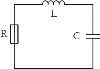
Figure 1. The RLC series circuit.
Download figure:
Standard image High-resolution imageAccording to the Kirchhoff's voltage law, we get

rearrange this equation and taking into account  , the following HE is obtained as

with  ,
,  , and
, and  , where
  is the initial charge value at t = 0,
  , and
, and  .
.
3. The analytical solution for the integrable case
The general form of the damped and nonlinear quadratic HE with arbitrary initial conditions could be written in the following form of initial value problem (IVP)

If the damped term is neglected  , the following undamped nonlinear HE is obtained

and for solving equation (19), the following ansatz is introduced

and by inserting equation (20) into (19), we get a system of algebraic equations and by solving this algebraic system with the help of initial conditions, we get

Using the initial conditions  , the values of
  and g3 can be estimated as

and

Now, let us consider the damped case (γ ≠ 0) and taking into account (20), the following new ansatz is considered

with Bfg ≠ 0 where f ≡ f(t) and g ≡ g(t).
The Weierstrass elliptic function ℘ ≡ ℘(f; g2, g3) is a solution to the following ordinary differential equation (ODE)

so that

Inserting ansatz (24) into equation (18) with the help of equation (26), we get  ,
,

Equating all coefficients of ℘j
and  to zero, the following system of ODEs is obtained
The compatibility conditions read
and by solving system (28), we get
As is well known, equation (18) is generally non-integrable except in some special cases e.g. α = 24γ2/25, it becomes integrable. Thus, the exact solution to equation (18) for α = 24γ2/25, is given by
where δ = ± 1 and the values of the constants c1 and c2 can be estimated by applying the initial conditions  and they are given by

and
The exact analytical solution of IVP (18) could be expressed in terms of the Weierstrass function as shown in equation (30). In addition to, the solution (30) could be written in the form of the Jacobian elliptic cosine function cn. To do that, let us introduce the relation between the Weierstrass and Jacobian elliptic functions (the details of the relation are omitted here)
This relation is true and both sides are equivalent.
Using relation (33) in the solution (30) and after several simple mathematical operations, we can arrive to the following solution in the form of Jacobian elliptic function cn
Note that both solutions (30) and (34) satisfy the IVP (18), i.e. the both solutions are equivalent. Moreover, the solution (30) covers solution (71) in [8] for g3 = 0, β = −β, and α = 6δ2/25 which means that the two solutions are true and satisfy the IVP (18).
In general and for any values for g2 and g3, the solution of the IVP (18) in the form of Jacobian elliptic function cn has the following formula
for m ≠ −1/4 and any value for A and the values of both g2 and g3 are given by
It must be noted here that the necessary condition for equation (18) to be integral is α = 24γ2/25 and otherwise, i.e. if α ≠ 24γ2/25, then equation (18) becomes non-integrable and in this case, we will try to find an approximate analytical solution for non-integrable case in the next section.
4. The approximate solution for the non-integrable case
Generally, for solving equation (18), the following ansatz is introduced

In order to estimate the values of  ,
,  , g2, and g3, we try to solve the following system of algebraic equations

where

After straightforward and manipulations, the following values are obtained


and
Now, in order to obtain an approximate solution obeying the initial conditions, we assume an ansatz of the form
where the values of the constants c0 and c1 can be obtained by applying the initial conditions and the following system is obtained
by solving system (45), we get

Finally, the value of ρ can be determined from the following condition

where q is given by (44).
Inserting the values of  ,
,  ,
,  , g2, g3, c0, and c1 that are given in equations (39)–(46) into (37), we finally obtain the thirteenth degree equation for ρ as

where the value of dj (j = 0, 1, ⋯ 11) is given in the appendix.
It should be mentioned that we will choose ρ to be the real root of (48). Thus, we may choose ρ = 4/5γ as default value.
5. Results and discussions
5.1. Example 1 (electronic applications)
In what follows, we first consider the case of  and positive value for β by considering the RLC circuit with R = 1 Ω, L = 2 H, C = 0.5 mF, q0 = 2C, and
  According to these data, the values of the following parameters are estimated

and the semi-analytical solution (36) reads
Figures 2(a)–(c) demonstrate the comparison between the semi-analytical solution (50) and the approximate numerical solutions via using Runge–Kutta fourth-order (RK4), FDM, and HPM the first-two approximations, respectively. It is observed that due to the presence of ohmic resistance R, the energy losses and dissipation occurs during this resistance which leads to the damping oscillations as shown in figure 2. Also, it is observed that the results produced by our semi-analytical solution (50) are in a very good agreement with the numerical solutions. Also, the maximum distance errors between the semi-analytical solution (50) and the approximate numerical solutions by using RK4, FDM, and HPM are, respectively, estimated as


and

These results confirm the high accuracy of our approximate analytical solution (36) or (44) as compared to the RK4, FDM, HPM approximate numerical solutions. Also, it is observed that the semi-analytical solution (50) is more accurate than the approximate numerical solution obtained by the HPM but it is similar to FDM in the accuracy.
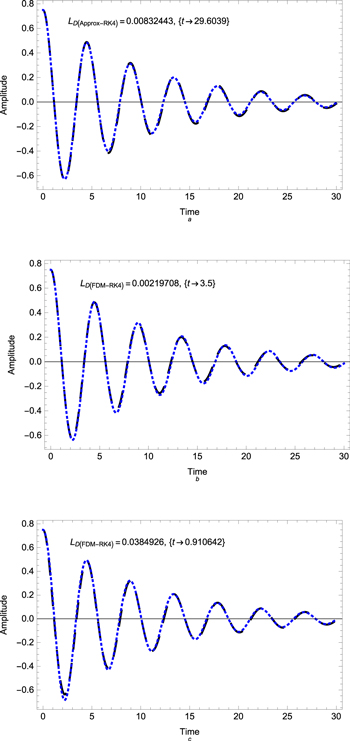
Figure 2. A comparison between the semi-analytical solution (36) (dashed curve) and (a) the RK4 numerical solution (dotted curve), (b) the FDM numerical solution (dotted curve), and (c) the HPM numerical solution (dotted curve). Here, α = 2, β = 0.2, γ = 0.1, q0 = 3/4, and  .
.
Download figure:
Standard image High-resolution imageNow, we consider the case of  and negative value for β as:

According to these data equation (36) can be summarized as
Figures 3(a)–(c) show a comparison between the semi-analytical solution (55) and the approximate numerical solutions via using the RK4, FDM, and HPM, respectively. Over and above, the maximum distance errors between the semi-analytical solution (55) and the approximate numerical solutions are estimated, as


and

It is clear that the semi-analytical solution is more accurate than the approximate numerical solutions obtained by both the FDM and HPM.

Figure 3. A comparison between the semi-analytical solution (36) (dashed curve) and (a) the RK4 numerical solution (dotted curve), (b) the FDM numerical solution (dotted curve), and (c) the HPM numerical solution (dotted curve). Here, α = 3, β = −0.25, γ = 0.2, q0 = 1 , and  .
.
Download figure:
Standard image High-resolution image5.2. Example 2 (plasma physics applications)
Now, we can use our solutions to investigate the damped oscillating in the present plasma model. In this model, the following experimental data [36, 37] are considered: electron temperature is given by Te
≈ 0.69 eV and the negative ion temperature reads  eV while ne
= 3.8 × 109 cm−3 gives the electron number density which these data lead to σ−i
= 8.7, 11.5, and 17.25, 0 ≤ μ−i
≤ 1 donates the negative ion concentration range, the dust concentration range is given by 0 ≤ βd ≤ 0.5 [37–40] and the value of
eV while ne
= 3.8 × 109 cm−3 gives the electron number density which these data lead to σ−i
= 8.7, 11.5, and 17.25, 0 ≤ μ−i
≤ 1 donates the negative ion concentration range, the dust concentration range is given by 0 ≤ βd ≤ 0.5 [37–40] and the value of  . Accordingly and for the relevant plasma parameters
  , the following values of Helmholtz parameters α, β, and γ are obtained: α = 0.77 813, β = 0.0721 875, and γ = −0.048 633 and solution (36) reduces to
Also, the maximum distance errors with the approximate numerical solutions are calculated as


and

By representing these data graphically according to the solution (59) and approximate numerical solutions, we can see concretely the perfect fit between both solutions as elucidate in figure 4. Also, we can note that the semi-analytical solution is more accurate than the HPM solution but maybe similar to the FDM accuracy.
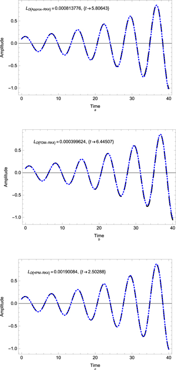
Figure 4. A comparison between the semi-analytical solution (36) (dashed curve) and (a) the RK4 numerical solution (dotted curve), (b) the FDM numerical solution (dotted curve), and (c) the HPM numerical solution (dotted curve). Here, the values of the physical parameters are subject to the presnt plasma model: α = 0.77 813, β = 0.0721 875, γ = −0.048 633, q0 = 0.1, and  .
.
Download figure:
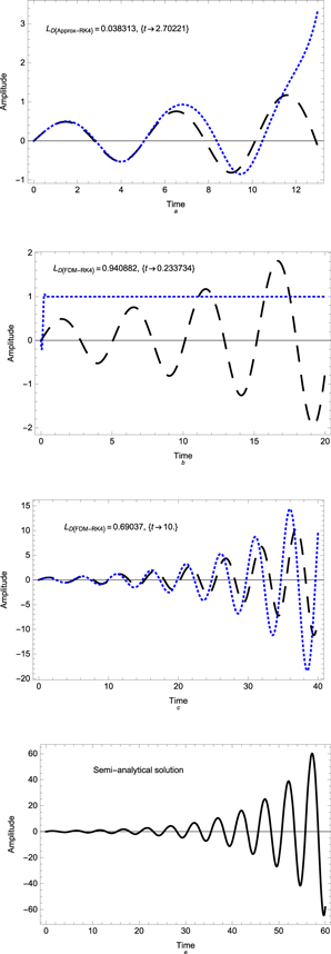
Standard image High-resolution imageFor the relevant plasma parameters  , the following values of Helmholtz parameters α, β, and γ are obtained: α = 1.61 776 663, β = −0.892 012, and γ = −0.1 and solution (36) can be written in the form
and the maximum distance errors with the approximate numerical solutions by using RK4 and FDM are given by


and

It clear from figure 5 that the numerical solution gives bad results for large time as compared to our solution (63) which demonstrates that our new approach is more robust. However, for small time, the numerical and analytical approximate solutions are largely consistent. Also, it is seen from the maximum distance errors (64)–(66) that the semi-analytical solution is more accurate than all approximate numerical solutions (RK4, FDM, and HPM). Moreover, the approximate numerical solution of HPM is more accurate than both the RK4 and FDM in this example. We can conclude that our semi-analytical solution is more accurate and stable with any time values and better than the numerical solutions.
Figure 5. A comparison between the semi-analytical solution (36) (dashed curve) and (a) the RK4 numerical solution (dotted curve), (b) the FDM numerical solution (dotted curve), (c) the HPM numerical solution (dotted curve), (d) he semi-analytical solution (36) (solid curve). Here, the values of the physical parameters are subject to the presnt plasma model: α = 1.61 776 663, β = −0.892 012, γ = −0.1, q0 = 0 , and  .
.
Download figure:
Standard image High-resolution image
6. Conclusions
The (un)damped nonlinear Helmholtz oscillator problem has been solved analytically through the Weierstrass elliptic function. In our analysis and for the first time, we used a new assumption (or ansatz (44)) to find an approximate analytical solution to the Helmholtz oscillator problem. Also, we obtained a necessary and sufficient condition for the integrability of the damped Helmholtz oscillator using an elementary approach which it did not use in the hard theory of Lie groups [8]. This urged us to look for an approximate analytical solution to the non-integrable case. The approach that has been used in present paper may be useful in studying and investigating the characteristics behavior of various nonlinear problems that were described by a DE of the form z'' = F(z) in the sense that z = z(t) may be approximated by an appropriate solution of Helmholtz oscillator by replacing F(z) by a suitable second degree polynomial in z. As a real application for the obtained solution, we applied our solutions on the signals that can propagate in the RLC series circuits for different values of its inductance L, resistance R, and the capacitance C. Moreover, the govern equations of the fluid complex plasma particles have been reduced to the KdVB equation using the RPM and this equation has been converted to the damped HE via using a suitable transformation. Posteriorly, the obtained solutions have been applied to investigate the behavior of wave oscillations versus the plasma parameters. It is observed from the numerical results that the approximate analytical solution is nearly closed to the analytical solution. Moreover, the maximum distance error for the approximate analytical solution as compared to the RK4 method, the FDM, HPM has been examined. It is found that the obtained results are of high accuracy and are largely consistent with the numerical results. Also, in some cases and for any time interval, the semi-analytical results are superior to the all numerical solutions, as is evident in the second example of the plasma.
Future work, using the Weierstrass elliptic function for studying the damped and undamped Helmholtz/Duffing oscillators problem with external constant and periodic force is considered a vital and important problem in many physical applications but out of the present scope [43].
Acknowledgments
Taif University Researchers Supporting Project number (TURSP-2020/275), Taif University, Taif, Saudi Arabia.
Appendix
and
