

Abstract
The Atacama Millimeter/submillimeter Array (ALMA) Phasing Project (APP) has developed and deployed the hardware and software necessary to coherently sum the signals of individual ALMA antennas and record the aggregate sum in Very Long Baseline Interferometry (VLBI) Data Exchange Format. These beamforming capabilities allow the ALMA array to collectively function as the equivalent of a single large aperture and participate in global VLBI arrays. The inclusion of phased ALMA in current VLBI networks operating at (sub)millimeter wavelengths provides an order of magnitude improvement in sensitivity, as well as enhancements in u–v coverage and north–south angular resolution. The availability of a phased ALMA enables a wide range of new ultra-high angular resolution science applications, including the resolution of supermassive black holes on event horizon scales and studies of the launch and collimation of astrophysical jets. It also provides a high-sensitivity aperture that may be used for investigations such as pulsar searches at high frequencies. This paper provides an overview of the ALMA Phasing System design, implementation, and performance characteristics.
Export citation and abstract BibTeX RIS
1. Background
The technique of Very Long Baseline Interferometry (VLBI) provides measurements of astronomical sources with the highest angular resolution presently achievable. At centimeter wavelengths, VLBI has been used since the 1960s to measure the sizes and structures of radio sources on scales finer than a milliarcsecond (see Kellermann & Cohen 1988; Walker 1999). Extension of VLBI techniques to the millimeter (mm) regime brings into reach still higher angular resolution—as fine as a few tens of microarcseconds. VLBI at mm wavelengths is also uniquely powerful in enabling the study of sources that are scatter-broadened or self-absorbed at longer wavelengths (e.g., extragalactic radio sources and supermassive black holes; Krichbaum 1996; Doeleman et al. 2008; Hada et al. 2013; Boccardi et al. 2016), or that emit high brightness temperature emission from spectral lines in mm bands (e.g., Doeleman et al. 2002, 2004; Richter et al. 2016; Issaoun et al. 2017).
The successful expansion of VLBI into the mm domain during the 1980s required both technological advances and the development of special algorithms to overcome the challenges posed by the decreasing atmospheric coherence timescales at shorter wavelengths (Rogers et al. 1984, 1995; Johnson et al. 2015). The first successful VLBI experiments at wavelengths as short as ∼1 mm involved only a single baseline (Padin et al. 1990; Greve et al. 1995; Krichbaum et al. 1997). Various experiments over the decade that followed met with mixed success owing to the small bandwidths that could be observed with the analog systems of the era. The development and deployment of digital backends (DBEs) and new recording systems based on hard drives (namely the Mark 5 recording systems; Whitney et al. 2010) provided a much-needed boost in sensitivity. These and other technical developments culminated in 2007 with the first detection of Schwarzschild radius–scale structure in Sagittarius A* (Sgr A*) at 1.3 mm on baselines from the Arizona Radio Observatory's Submillimeter Telescope to the James Clerk Maxwell Telescope and a telescope of the Combined Array for Research in Millimeter-wave Astronomy (CARMA; Doeleman et al. 2008). Motivated by this success, the 1.3 mm observing array, known as the Event Horizon Telescope (EHT; Doeleman et al. 2009), was expanded over the following years to include the Submillimeter Array (SMA), the Institut de Radioastronomie Millimétrique (IRAM) 30 m telescope, the Atacama Pathfinder EXperiment (APEX), the Large Millimeter Telescope Alfonso Serrano (LMT), and the South Pole Telescope, along with the now-defunct Caltech Submillimeter Observatory. Key results from these observations included the detection of ordered magnetic fields in an asymmetrically bright emission region around Sgr A* (Johnson et al. 2015; Fish et al. 2016) and very compact structure at the base of the jet from the supermassive black hole in M87 (Doeleman et al. 2012).
Despite these successes, the use of mm VLBI techniques has been restricted to the study of a relatively small number of bright sources owing to the limited sensitivity of existing networks of VLBI antennas. This is a consequence both of higher receiver noise and the relatively small apertures (or effective apertures) of most telescopes operating at frequencies of ≳100 GHz. Furthermore, at wavelengths shorter than 3 mm, the small number of suitably equipped VLBI stations have offered too few baselines to allow sources to be imaged (e.g., Doeleman et al. 2009).
As a major step toward overcoming these limitations, the ALMA Phasing Project (APP) was conceived with the goal of harnessing the extraordinary sensitivity of the Atacama Large Millimeter/submillimeter Array (ALMA) for VLBI science. While capturing data from each separate ALMA antenna is neither practical nor desirable, ALMA can be used as a single large-aperture VLBI antenna if the data from its individual antennas are phase-corrected and coherently added together. The goals of the APP were to provide the hardware and software necessary to perform these operations and to record the resulting data in VLBI format.
Phased arrays have been used as VLBI stations at centimeter wavelengths since the late 1970s, beginning with the Westerbork Synthesis Radio Telescope (e.g., Kapahi & Schilizzi 1979; Raimond 1996; Schilizzi & Gurvits 1996), and also including the phased Very Large Array (VLA; e.g., Wrobel 1983; Lo et al. 1985) and the phased Australia Telescope Compact Array (e.g., Tzioumis 1997). More recently, phased arrays, including the Plateau de Bure,16 SMA, and CARMA, have also been deployed for VLBI in the mm regime (e.g., Krichbaum et al. 2008; Weintroub 2008). Some of the factors affecting the performance and efficiency of these earlier phased arrays have been discussed by, e.g., van Ardenne (1979, 1980), Ulvestad (1988), Dewey (1994), Moran (1989) and Kokkeler et al. (2001).
An optimally phased array provides a collecting area equivalent to the combined effective area of the individual antennas, thereby boosting the achievable signal-to-noise ratio (S/N) of VLBI baselines to the site. The addition of a phased ALMA to existing VLBI networks operating at mm wavelengths therefore has the ability to offer up to an order of magnitude boost in sensitivity. For many experiments, the geographical location of ALMA also provides a significant improvement in u–v coverage, dramatically enhancing the ability to reconstruct images of sources. And when used in conjunction with the Global mm-VLBI Array (GMVA) at 3 mm, ALMA will also provide a factor of two improvement in north–south angular resolution. Figure 1 illustrates the geographic distribution of some of the VLBI antennas currently available to operate in conjunction with ALMA at wavelengths of 1 mm and/or 3 mm. The 1 mm observing sites are part of the EHT, as described above. The GMVA sites include eight stations of the Very Long Baseline Array (VLBA), along with the Robert C. Byrd Green Bank Telescope (GBT), the Effelsberg 100 m Radio Telescope, the Yebes Observatory 40 m telescope, the IRAM 30 m telescope, the Metsähovi 14 m telescope, and the Onsala Space Observatory 20 m telescope. Additional EHT and GMVA sites are expected to become available during the next few years.
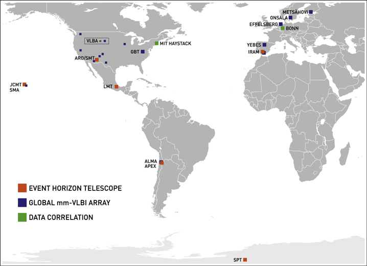
Figure 1. Map showing the global distribution of stations operating in conjunction with phased ALMA for VLBI during ALMA Cycles 4 and 5. Sites with Band 6 (1 mm) capabilities (part of the EHT) are shown in red; stations with Band 3 (3 mm) capabilities (part of the GMVA) are shown in blue; correlation centers (see Section 6) are shown in green. Sites that are part of the VLBA are not individually labeled and are distinguished from the other GMVA sites by a smaller symbol.
Download figure:
Standard image High-resolution imageThe science case for a beamformed ALMA, described in detail by Fish et al. (2013) and Tilanus et al. (2014), is broad and diverse. VLBI observations of supermassive black holes on event-horizon scales can be used to gain a better understanding of the astrophysics of accretion in black hole systems and to test predictions of General Relativity. High-resolution imaging of the jet launching, acceleration, and collimation regions in active galactic nuclei will illuminate how jets are formed, and exquisitely detailed studies of the nearest extragalactic jets, such as the one in M87, will provide a benchmark for the general understanding of jet physics (e.g., Asada & Nakamura2012; Asada et al. 2014).
High-frequency pulsar observations enabled by a phased ALMA (see also Section 9) will aid our understanding of pulsar emission processes, and pulsar searches in the Galactic Center may uncover a system that can be used for relativistic tests at very high precision. (Sub)mm maser observations at VLBI resolutions can be used to better understand the physical conditions in star-forming regions, evolved stars (on au scales), and the circumnuclear environment of other galaxies, and multi-epoch observations of maser sources have the potential to provide higher astrometric accuracy than has been possible previously. In addition, new observations of absorbing systems at cosmological distances are poised to provide information on the physical conditions of the early universe and chemical evolution over time and can also be used to test for variability of fundamental physical constants.
The initial implementation of the ALMA Phasing System (APS) focused on the simplest use case: continuum VLBI on sources bright enough to allow on-source phasing of the array. To date, the APS has been commissioned and approved for science observations in Bands 3 and 6 (corresponding to wavelengths of 3 mm and 1.3 mm, respectively), where the GMVA and the EHT, respectively are available to serve as the respective partner networks (Figure 1). The first science observations that included the APS in this capacity were conducted in 2017 April as part of ALMA Cycle 4.
The outline of this paper is as follows. We first briefly summarize some of the attributes of the ALMA array relevant to its use as a VLBI station (Section 2). In Section 3, we provide an overview of the APS and subsequently describe in more detail the hardware (Section 4) and software components (Section 5) developed by the APP team to enable operation of ALMA as a phased array and a VLBI station, as well as the specialized procedures required for correlation of the resulting data (Sections 6 and 7). In Section 8 we describe some of the performance characteristics of phased ALMA derived from on-sky commissioning and science verification (CSV). Finally, in Section 9, we briefly describe enhancements of the APS that are being developed to expand the breadth of its scientific capabilities.
2. The Transformation of ALMA into a VLBI Station
ALMA is currently the world's largest and most sensitive facility devoted to mm and sub-mm astronomy (e.g., Wootten & Thompson 2009). The ALMA array, located on the Chajnantor Plateau in the Atacama desert of northern Chile, comprises 66 reconfigurable antennas, twelve of which are 7 m diameter parabolic dishes arrayed in a closely spaced configuration and 54 of which are 12 m diameter parabolic dishes. The antennas, as well as the ALMA baseline (BL) correlator, the ALMA Compact Array (ACA) correlator, and the Central Local Oscillator are located at the Array Operations Site (AOS) at an elevation of approximately 5000 m, while science operations are conducted from an Operations Support Facility (OSF) at 2900 m.
Antenna baselines within the ALMA array can range from ∼9 m (within the ACA) to 16 km, depending on the array configuration. However, relatively compact configurations (where most antennas are on baselines of ≲1 km) are the most desirable for phased array operations, since decorrelation of signals caused by variations in the atmosphere above each of the antennas is minimized.
Fifty of ALMA's 12 m antennas comprise the so-called "12 m Array," which in its standard operating mode is used in conjunction with the 64-antenna BL correlator as a connected element interferometer to perform sensitive, high-resolution imaging observations. The sixteen remaining antennas (twelve 7 m antennas and four 12 m antennas) comprise the ALMA "Compact Array," which can be operated using a separate, independent ACA correlator for the purpose of obtaining total power measurements and enhanced imaging of extended sources or large-scale structures. Antennas from the ACA may also be correlated by the BL correlator along with antennas from the 12 m Array.
With an outlook toward future enhancements to ALMA's capabilities, the ALMA BL correlator (Escoffier et al. 2007) was designed with "hooks" to allow future VLBI observations (Baudry et al. 2012; see Section 4.2). Importantly, the BL correlator was designed to carry out these additional operations while at the same time performing the usual correlation of signals from the individual baselines. The APS was conceived to take advantage of this framework and provide the additional hardware and software components necessary to operate ALMA as a phased array and record the resulting data streams in a standard VLBI format.
3. Overview of the APS
An antenna phasing system intended to operate at mm (or sub-mm) wavelengths must be designed to accommodate the unique challenges of observing at these wavelengths, including atmospheric attenuation and the rapid fluctuations in the signal phases from astronomical sources caused by tropospheric water vapor (e.g., Carilli et al. 1999). These factors are important even at a superb observing site such as ALMA's. An additional consideration for the phasing system at ALMA was that, at minimum, it would be capable of meeting the needs and goals of mm VLBI experiments that require an order-of-magnitude improvement in sensitivity for continuum observations compared with existing capabilities.
The aforementioned goals led to a set of functional requirements for the APS that included: (1) ability to phase up and sum up to 61 antenna signals; (2) a capability for real-time assessment of phasing performance; (3) ability to apply rapid phase adjustments based on data from water vapor radiometers (WVRs); (4) VLBI-quality frequency stability and timing; (5) full bandwidth, dual polarization VLBI recording; (6) circularly polarized data products (as required to facilitate VLBI data analysis); and (7) ≥90% phasing efficiency. In practice, requirement (7) needed to be relaxed for end-to-end operations (see Section 8.2). On-sky testing and verification of the system to validate it against these various formal requirements are discussed in Section 8. As described in Section 9, provisions were also made for additional features that could be implemented at a later date.
Another important consideration was the need to design and deploy the phasing system and ALMA VLBI capabilities without impacting normal ALMA operations. Furthermore, it was required that scientifically valid standard interferometry data from the ALMA BL correlator be archived in parallel during APS operations, independent of the VLBI recordings.
The APS block diagram is shown in Figure 2, and some of the key characteristics of the integrated APS are summarized in Table 1. In Figure 2, the green blocks group together elements into the three main areas of hardware and software enhancements to ALMA: (i) frequency stability ("Maser"); (ii) data formatting, transport, and recording ("VLBI"); (iii) the beamforming of the array ("Phasing"). The phasing or "beamforming" component of the APS analyzes the visibilities from the BL correlator to compute phase adjustments to the individual antennas (Section 5). This allows the formation of coherent sum signals which are provided to specially designed phasing interface cards (PICs) in the BL correlator (Section 4.2). At the same time, these signals are sent through the BL correlator as if they came from an ordinary ALMA antenna so that the performance of the system may be monitored in real time.

Figure 2. Diagram of the APS, illustrating how existing ALMA systems were modified to support VLBI. Pre-existing objects are shown in pink and objects in blue are new components added by the APP. The green backgrounds group related components.
Download figure:
Standard image High-resolution imageTable 1. Characteristics of the ALMA Phasing System
| Feature | Specification | Remarks |
|---|---|---|
| Number of phased antennasa,b |

|
Number of phased antennas must be odd. |
| Equivalent collecting area | 4185 m2 | Assuming 37 phased 12 m dishes and neglecting efficiency lossesb. |
| Frequencies of operationc | ALMA Bands 3 and 6 | Extension to Bands 1 and 7 anticipated for ALMA Cycle 7. |
| Effective bandwidth per quadrant | 1.875 GHz | Four quadrants total; see Section 4.2. |
| Effective aggregate bandwidth | 7.5 GHz | Per polarization. |
| VLBI recording speedd | 64 Gbps | 4 Mark 6 units, each 16 Gbps; dual linear polarizations recorded; 2-bit sampling |
| SEFDe | 65 Jy (at 3 mm) | Assuming 37 phased 12 m antennas.b |
| 97 Jy (at 1.3 mm) | ⋯ | |
| Phasing efficiencyf | ∼60% | Empirically derived value, including all measured efficiency losses. |
| Flux density threshold for phasingg | ≳0.5 Jy | For Bands 3 and 6 in ALMA Cycles 4 and 5. |
Notes.
aThe maximum is set by the design of the ALMA BL correlator (Section 4.2) and the practice of designating at least two antennas unphased comparison antennas (Section 5.2.1). bThe anticipated number of antennas available for phasing during ALMA Cycle 5 is ∼37. cThe APS was commissioned for use in ALMA Bands 3 and 6. However, it is capable of operation in any band provided that weather conditions are suitable. dThe maximum recording rate available at ALMA's VLBI partner sites during ALMA Cycle 4 was 2 Gbps for the GMVA and 32 Gbps for the EHT. In Cycle 5, this rate is expected to increase to 64 Gbps for the EHT sites. eThe system equivalent flux density (SEFD) for Band 3 assumes an aperture efficiency of 0.71 and a typical zenith system temperature of 70 K; for Band 6, the SEFD assumes an aperture efficiency of 0.68, and a zenith system temperature of 100 K. fSee Section 8.2 for discussion. gImprovements in the handling of delays (Section 5.2.4) will enable direct phase-up on weaker sources, while a future passive phasing mode (Section 9) will enable VLBI on sources too weak for phasing.Download table as: ASCIITypeset image
In general, a VLBI DBE takes the native analog receiver signals, downconverted to an intermediate frequency (IF), digitizes them, and converts them to a standard data format (in this case, VLBI data interchange format or "VDIF")17 to allow future playback at the VLBI correlators (Section 6). At ALMA the signals originate in the BL correlator at the AOS, and the PICs serve as the VLBI backend, translating the ALMA digital signals into VDIF packets (Section 4.2). These signals are brought down to the ALMA low site (OSF) on an Optical Fiber Link System (OFLS; Section 4.4) to the VLBI recorders (Section 4.3).
All phasing operations in the APS are performed entirely in software. The green fields in Figure 3 delineate the three domains of software activity required: (i) Phasing; (ii) VLBI Recording; and (iii) Maser Control. Modifications to the original ALMA software allow it to provide software "devices" to control and monitor all of the new VLBI hardware, as well as new "controllers" to manage the operations of these parts of the system. One of these, the InterferometryController, is the same one that runs standard (connected element) interferometry observations during normal (non-VLBI) ALMA operations. The phasing system itself is managed by a PhasingController (Section 5.2.1) that directs the BL correlator hardware to make phasing adjustments based on calculations made in the Telescope Calibration System (TelCal), which is the ALMA software component that provides all online observatory calibration reductions. A VLBIController (Section 5.1) is also introduced to manage the VLBI activities of the observation; it operates independently of the PhasingController. Figure 3 also shows the software required to interface between the "Schedule Block" normally used to execute ALMA observations, with the VLBI EXperiment (VEX) file paradigm that is a community standard for the execution of VLBI observations (Section 5.2.5).
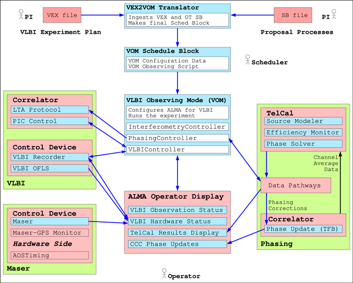
Figure 3. Diagram of the APS software, highlighting the new components added to support VLBI. Objects in pink previously existed; objects in blue are new and were developed as part of the APP. The green backgrounds group related components.
Download figure:
Standard image High-resolution imageA subsequent stage of VLBI operations is the VLBI correlation, which is performed after the observations at specialized VLBI correlators using time-stamped data recorded at ALMA and other observatories (Section 6). The VLBI correlation is analogous to the role played by the ALMA BL correlator during standard interferometry, but where data from the global VLBI telescopes are processed instead of data from the connected ALMA elements. However, the time stamping for VLBI requires nanosecond (ns) precision, which is derived from a frequency-stabilized hydrogen maser that was purchased for this purpose and adapted to meet all of ALMA's timing needs (Section 4.1).
4. APS Hardware
Implementation of beamforming and VLBI capabilities at ALMA entailed installation of four new major hardware components at ALMA: (1) a hydrogen maser to serve as a frequency standard; (2) BL correlator modifications that included: (i) installation of PICs to serve as the VLBI backend and (ii) installation of an additional card to serve as a 1 pulse-per-second (1 PPS) signal distributor to the PICs; (3) a bank of four high-speed VLBI recorders; (4) an optical fiber link system (OFLS) to carry the data stream from the ALMA correlator at the ALMA AOS to the recorders at the ALMA OSF. We now describe each of these components in more detail.
4.1. Maser
VLBI depends on the fundamental ability of radio receivers to accurately preserve the phase of astronomical signals by referencing them to an independent frequency standard at each of the participating VLBI stations. Prior to the APP, the ALMA array, when operating as a connected element interferometer, depended on a common local oscillator (LO) derived from a 5 MHz rubidium (Rb) clock. However, the Rb clock does not meet the strict stability requirements for a VLBI frequency standard, namely that the rms phase fluctuations are kept well below one radian. This condition may be expressed as  , where ω is the LO frequency in rad s−1,
  is the Allan standard deviation (equal to the square root of the Allan variance), and t is the integration time in seconds (Rogers & Moran 1981).
Because of their superb stability on timescales comparable to VLBI integrations, hydrogen masers are used almost exclusively as frequency references for VLBI. At mm wavelengths, tropospheric turbulence limits typical VLBI integration times to ∼10 s. Since modern hydrogen masers achieve  , VLBI observations at wavelengths of ∼1 mm can be carried out with coherence losses of
  (Doeleman et al. 2011). To fulfill this need at ALMA, a commercially available T4 Science iMaser was purchased and installed in a seismic rack at the ALMA AOS as part of the APP. ALMA's Rb clock was also kept in place as a hot spare for use in non-VLBI observations, but the hydrogen maser is now the default frequency standard for all ALMA observing modes.
The original APS design called for a straightforward repla-cement of the 5 MHz Rb reference with a 5 MHz output from the hydrogen maser. However, it was found that to preserve the required VLBI stability and phase noise specifications for the ALMA receiver LO signals, both the 5 MHz and 10 MHz outputs of the hydrogen maser had to be utilized. This required a minor modification of the ALMA Central Reference Generator, but the capability of switching back to the Rb clock as a hot spare for non-VLBI observations was preserved.
The hydrogen maser at ALMA is routinely monitored in two ways. With the first method, the stability of the maser's 10 MHz signal is compared with that of a high-precision quartz oscillator. The crystal is not as good as the maser over long periods, but it is of comparable stability over ∼1 s intervals (where the maser signal is also conditioned by a crystal). Results of such a comparison are shown in Figure 4.
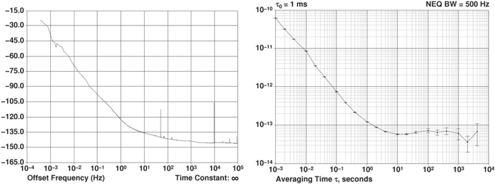
Figure 4. Left: phase noise in units of dBc Hz−1 as a function of offset frequency in Hz based on a comparison between the hydrogen maser installed at the ALMA AOS and a precision quartz oscillator. Right: Allan deviation between the maser and the same quartz oscillator as a function of averaging time in seconds. For a 1 s average, the Allan deviation for the ALMA maser alone is  times the value measured between the two devices, i.e.,
  , which matches the required specification (see Section 4.1 for details).
Download figure:
Standard image High-resolution imageThe left panel of Figure 4 shows a phase noise comparison between the ALMA maser and an Oscilloquartz 8607 quartz oscillator. The phase noise specification for the maser is −124 dBc Hz−1 at 1 Hz from the 10 MHz reference. In a comparison of two oscillators with similar noise characteristics, one expects to measure a value that is 3 dBc Hz−1 higher, and the phase noise plot confirms the maser is operating at specification or better. The right panel of Figure 4 is the measured Allan deviation,  , between the hydrogen maser and the same quartz oscillator, both of which should have similar stability over 1 s integrations. The measured value of the Allan deviation of
  at 1 s for two similar oscillators, implying that the Allan deviation for the maser alone is
  (i.e.,
  times the value measured for the two oscillators), which matches the required specification.
A second type of maser health check involves routinely monitoring the offset between the 1 PPS signal generated by the maser from its 10 MHz output with another 1 PPS signal generated by a global positioning system (GPS) receiver. GPS stability on 1 s timescales is poor due to variations induced by the ionosphere and will vary by a few tens of nanoseconds on a diurnal cycle due to ionospheric total electron content (TEC) changes. However, on longer timescales ( s), GPS is providing an average time rate synchronized with the United States Naval Observatory timekeeping for Coordinated Universal Time (UTC) and its precision will exceed that of a single hydrogen maser. If the maser is operating properly, a plot showing a comparison of the two signals is expected to show a linear drift at a rate characteristic of the maser, with some arbitrary offset due to the initialization of the first maser 1 PPS pulse. A plot of the residuals to such a linear fit for the ALMA maser is shown in Figure 5 for the period leading up to the 2017 April VLBI campaign at ALMA. It shows several weeks of data, with fits on ≈10 day intervals (designated in different colors). Prior to the campaign, the maser was "tuned" by adjusting the digital synthesizer which generates the 10 MHz oscillation for zero drift relative to UTC. Several fits over the final two-week period suggest that the average drift was essentially zero, with a measurement uncertainty of fs s−1.

Figure 5. Timekeeping from the ALMA hydrogen maser relative to a GPS as a function of time. Residuals to linear fits to the data, grouped in approximately 10-day intervals (differentiated by color), are plotted for several weeks of data leading up to the ALMA Cycle 4 VLBI campaign in 2017 April. These results show that there was negligible drift in the maser over this interval.
Download figure:
Standard image High-resolution image4.2. Baseline (BL) Correlator Modifications
The 64-antenna ALMA BL correlator processes four 2 GHz frequency chunks of dual-polarization spectrum from up to 64 antennas, one chunk per quadrant. Each data stream requires a PIC to serve as a VLBI backend and to transfer the ALMA signals to the VLBI recorders. In total, eight PICs are required (one per polarization in each of the four 2 GHz correlator quadrants).
The ALMA BL correlator has an "FXF" architecture (Escoffier et al. 2007). The 2 GHz input band is initially sliced into thirty-two 62.5 MHz pieces ("F") by sets of tunable digital filter bank (TFB) cards, whose design is described in Camino et al. (2008). Each 62.5 MHz "TFB channel" has an approximately flat response determined by the digital filter design implemented in the field programmable gate arrays (FPGAs) of each TFB card. These channels are overlapped slightly in frequency (15/16th of each channel), yielding an effective bandwidth is 1.875 GHz per quadrant. The TFB channels are processed in separate correlator "planes." The TFBs are followed by a hardware correlator ("X") and software Fourier transform ("F"). The correlator was designed with "hooks" for VLBI (Baudry et al. 2012), including spare card slots and rack space; extra power capability; a digital, high-resolution adjustment capability for the phases of the LOs in the TFBs (to 1/4096 of a 360° turn; see Figure 6); and FPGAs dedicated to computing a sum of a selectable set of antennas.
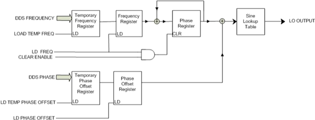
Figure 6. TFB Phase Adjustment Logic. In normal operation of each TFB, the logic in the upper half of this figure is active: the desired frequency is loaded and the contents of the phase register are cleared at the start of the observation. Thereafter the LO output is driven from a sine lookup table. When the APS is active, an additional 16 bit phase offset register is loaded with a value for the appropriate fraction of a turn of phase every correlator subscan in order to correct the phase of this TFB. This phase offset may be cleared (or not) at the start of a scan. The capability of leaving the phase offset register contents unchanged will enable a future use of a "passive" phasing mode (Section 9).
Download figure:
Standard image High-resolution imageThe BL Correlator has two modes of operation with regard to how the antenna signals are passed through the TFBs: time division mode ("TDM") and frequency division mode ("FDM"). TDM is the default for continuum observing with ALMA during standard interferometry observations; in this mode, the TFB cards are bypassed and the correlator behaves like a pure XF rather than an FXF system (Baudry et al. 2012). However, only FDM allows for phase adjustment of the TFBs and the option to easily capture channelized data in a VLBI data set.
In practice, the spectral specification allows one to define some number of channel averages (spectral sub-regions), which correspond to sets of TFBs, for the purpose of making phase adjustments. Because the employed FDM setup generates more ALMA standard interferometry data than can readily be archived in real time, some degree of spectrum averaging (typically a factor of eight) is used to reduce the volume of archived data.
The final design of the correlator modifications required for the APS is shown in Figure 7. Parts added for VLBI are shaded blue, with additional detail shown in yellow. Because timing precision and stability are critical to successful VLBI operations, a 1 PPS distribution system (card and cables) was installed to bring signals from the hydrogen maser (Section 4.1), as well as from a GPS unit, to the PICs so that the timing of the data in the packets could be continuously recorded against both of these signals (left side of Figure 7). The 1 PPS signal from the maser should be completely invariant in the data, since the entire ALMA system is operated from the maser 10 MHz output. On the other hand, as noted above, the 1 PPS signal from the GPS unit typically varies by tens of nanoseconds due to diurnal ionospheric TEC changes.
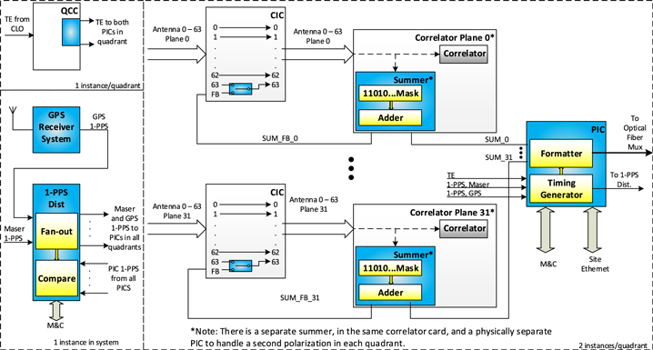
Figure 7. Block diagram of the ALMA BL correlator modifications required for the APS. Changes are shown with blue boxes. Timing is managed with Timing Events (TEs) every 48 ms. The Quadrant Control Cards (QCCs, upper left box) were modified to send these signals to the eight Phasing Interface Cards (PICs), as depicted along the right. To verify timing, an independent GPS receiver and distribution system for a 1 PPS signal (lower left) were added. In addition, a 1 PPS signal from the maser (Section 4.1) is distributed to each PIC. The Correlator Interface Cards (CICs; two are shown on the left side of the main box) received a logic switch in the gateware that switches Correlator Antenna Input (CAI) number 63 between a single ALMA antenna (normal operations) and the output of the summer logic in the Correlator Plane assemblies. The summer has a mask to determine which antennas contribute to the sum, and it adds the appropriate 2 bit signals and rescales them back to two bits for input at CAI 63. The sums are performed on a per tunable filter band (TFB) channel basis, with 32 TFBs per quadrant in each polarization (SUM_FB_0 ... SUM_FB_31).
Download figure:
Standard image High-resolution imageOne complicating factor in the adaptation of the ALMA BL correlator for VLBI is the fact that ALMA uses a 48 ms Timing Event (TE) instead of the VLBI standard 1 PPS signal as a timing epoch standard. For this reason, several redundant measures were designed to insure that the timing is correct. The maser 1 PPS signal, a GPS 1 PPS signal, and the site TE are connected to the Timing Generators in each of the eight PICs. By design, the TE is coincident with the 1 PPS signal at seconds 0, 6, ... 54 and is carefully distributed so that its rising edge is within the same 125 MHz clock cycle everywhere in the correlator. To synchronize the PIC 1 PPS signal, the real-time control computer sends a "synchronize" command to each PIC's Timing Generator just prior to the TE at second 0. The 1 PPS Distributor has the ability to cross-check all of the PIC-generated 1 PPS signals against both the GPS and maser 1 PPS signals.
The ALMA BL correlator contains 64 Correlator Antenna Inputs (CAIs), numbered 0 through 63. To support VLBI, the firmware on the Correlator Interface Cards (CICs) was modified by insertion of a logic switch that toggles the input at CAI #63 from a single ALMA antenna to a phased sum of the array antennas (see Figure 7). This allows the phased sum to be correlated against any individual array antenna, providing a means of validating that the summation is correct.
The sum signal itself is produced using the summer logic in the Correlator Plane assemblies (Figure 7). The analog sum logic (gateware) in the dedicated FPGAs on each Correlator Card was modified to properly scale the outputted digitized samples and produce 2 bit signals for the PICs and CIC feedback. The sum is formed on a per TFB channel basis using a mask-selectable set of  antennas, where the mask is user-defined and relayed to the system via the correlator control system.
The mask is required for multiple reasons. First, in order to faithfully represent the sum,  must be odd. The reason is that in the available hardware circuit, only two bits per antenna are available. This allows representation of the signal voltage (part of a Gaussian distribution) as one of four possible values (two positive and two negative states). Consequently, with an even number of antennas, the resulting sum can be exactly zero, which in turn cannot be represented by any of the four available states. The simplest solution is to impose the requirement that the number of antennas be odd. Because a "zero" state is in fact the most probable one for a sum of an even number of antennas, the S/N loss incurred by omitting one antenna from the phased sum is always smaller than would result from having signals end up in non-representable zero states. A second reason for the mask is that it is useful to hold some antennas apart from the sum signal; one or more of these may be used as "comparison antennas" to estimate the efficiency of the phasing system (Section 8.2). Finally, depending on the configuration of ALMA, antennas that are on long baselines (>1 km) may be excluded to help insure good phase stability across the selected array.
In addition to the Timing Generator discussed above, the PICs also include a formatter. The formatter takes 2-bit data streams from 32 of the Correlator Cards in each quadrant and for each polarization, integrates them into a VDIF-compliant data stream, and routes them to a 10 GbE interface. The VDIF data stream is packaged in User Datagram Protocol (UDP) packets onto a 10 Gbps optical fiber which is mated to the PIC using an SFP+ network adapter. The PIC formatter supports bandwidths from 62.5 MHz to 2 GHz in binary multiples of 62.5 MHz and can also produce several types of test patterns for troubleshooting.
4.3. Mark 6 VLBI Recorders
The Mark 6 VLBI recorder is the current offering in a long line of VLBI recording systems developed by the Massachusetts Institute of Technology (MIT) Haystack Observatory. It is commercially manufactured by Conduant Corporation. The Mark 6 is based on commercial off-the-shelf technology and open-source software. Data are recorded onto "modules" comprising banks of eight commercial-grade 3.5 inch hard disks inserted into a Mark 6 chassis. Typically the disks are "conditioned" prior to use to eliminate bad sectors and to verify their performance.
Mark 6 recording was initially demonstrated in 2012 (Whitney et al. 2013) and first adopted for astronomical VLBI use at ALMA. Figure 8 shows two of the Mark 6 recorders shortly after installation at the ALMA OSF. In the ALMA configuration, each recorder accepts two VDIF packet streams (one per polarization) on two optical network cables and writes data onto four disk modules at an aggregate rate of 16 Gbps. When all four ALMA basebands are in use, the total recording rate is 64 Gbps (2 GHz of bandwidth from each of four basebands, Nyquist sampled, 2 bits per sample, with dual polarizations).
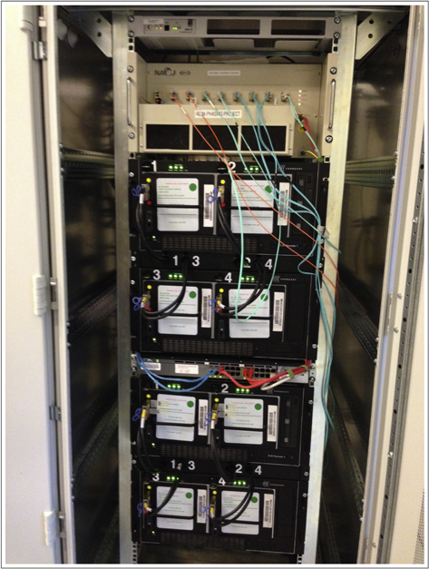
Figure 8. Recorders 1 and 4 installed in the designated ALMA OSF computer room rack. The OFLS unit is mounted at the top. Between the recorders is the network switch which connects the recorders to the AOS network and also provides a private network between the recorders.
Download figure:
Standard image High-resolution imageIn normal operations, there is some manual effort required to mount and unmount the disk modules and verify that these have survived the stress of international shipping. Thereafter the operation of the recorders is completely automatic at the ALMA Control system via the observing script and the VLBIController software.
The Mark 6 system development was concurrent with the APS development, and there were a number of issues to consider in adapting the recorder for use at ALMA. We needed to ensure that the capacity of the modules was sufficient to eliminate the need for module swaps during overnight VLBI observing shifts. Because the recorders were sited at the ALMA OSF (elevation 2900 m) in a climate-controlled computer room, some environmental issues relevant to other VLBI sites were not an issue. Nevertheless, we undertook extensive testing to verify that ordinary hard drives (rated for 10,000 ft) were indeed usable at ALMA.
In contrast to previous hard-disk VLBI recorders which used proprietary disk formats, we opted for an open, simple, non-RAID, "scatter-gather" plan for distributing data in ≈10 MB blocks across multiple disks. In practice, at ALMA the data from each PIC are thus spread over 16 disks so that a useful recording is still possible even in the event of network issues or disk failures. Finally, since the Mark 6 recorders are conventional Linux systems, it is possible to run DiFX correlation software (see Section 6) on the mini-cluster comprising the four recorders in order to perform local VLBI correlations of data. This was valuable for early testing, although in practice, the ability to routinely perform fringe tests with remote sites in near real time is precluded by the limited network bandwidth between ALMA and the other sites.
4.4. Optical Fiber Link System (OFLS)
An OFLS is required to transfer the antenna sum data generated by the APS from the ALMA AOS to the ALMA OSF where the VLBI recorders are located. The OFLS was designed by the National Astronomical Observatory of Japan and Elecs Industry Co. LTD. and fabricated by Elecs Industry. The system multiplexes the eight digital network streams generated by the PICs in the BL correlator (Section 4.2) onto a single ALMA fiber (out of a bundle of 48 fibers) for transmission. The measured signal loss ranges from ∼6–7 dB over the ∼30 km cable path. At the two ends, identical units multiplex the signals onto the single fiber with dense wavelength division multiplexing.
Each of the eight channels of the OFLS has a maximum data rate of 10 Gbps, allowing it to accommodate the data rate generated by each of the eight PICs (8 Gbps, plus a small overhead for the packet header of <1%). There is also a ninth channel available as a built-in spare, so in total there are 18 different data streams: nine downlink streams and nine uplink streams. The OFLS design is bi-directional since it is built based on 10GbE technologies, although the uplinks are not used during observations.
Figure 9 shows a schematic diagram of the OFLS. The data transfer through the single long-distance fiber is done with a 10GBASE-ZR optical module operating at a wavelength of 1550 nm. The optical channels designated  to
to  are assigned to the International Telecommunications Union (ITU) grids of 21, 23, 25, ..., 55, corresponding to frequencies of 192.1, 192.3, 192.5, ... 195.5 THz (i.e., 100 GHz spacing). In the OFLS the optical data are converted between 10GBASE-ZR and 10GBASE-SR so that the OFLS can interface the correlator PICs and Mark 6 recorders with 10GBASE-SR optical modules.
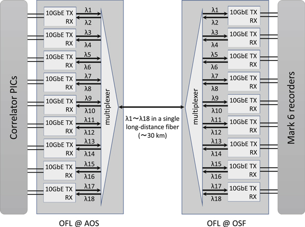
Figure 9. Schematic diagram of the optical fiber link system (OFLS), which connects the data stream generated by the BL correlator at the ALMA AOS with the Mark 6 VLBI recorders at ALMA OSF.
Download figure:
Standard image High-resolution imageSoftware connection to the OFLS and network control can be made with the VLBI Standard Interface for Software (VSI-S) protocol on a physical 10BASE-T/100BASE-T ethernet. For monitoring its status, the OFLS provides information such as power status, the link status of each channel, and temperature status. It has no packet monitoring capability, and thus it is a passive instrument in the VLBI phasing system. The OFLS was built with redundancy in terms of the number of cooling fans and DC power supplies to avoid failures in these parts, which tend to have relatively short mean times between failures (between a few to several years).
5. APS Software
5.1. The VLBI Controller and VLBI Observing Mode (VOM)
A VOM at ALMA is required to support the VLBI back end; this is handled by the VLBIController as indicated in Figure 3. By design, the VOM performs only limited functions: the PICs need to be programmed and the recorders need to be told what to record. For the PICs, programming consists of providing them with the VDIF header, which includes the number of channels to record and, critically, the timestamp for the data. As discussed in Section 4.2, the ALMA system is time-managed around TEs which occur every 48 ms. Every six seconds, one of these is coincident with an integral second, so one of these coincidences is chosen for the moment of programming: a VDIF header is downloaded prior to the TE and at the TE, the PIC starts its packaging and broadcasting of data. This stream is generated continuously until the correlator is reset or the PICs are turned off.
The data are only useful during the parts of the observing sequences when the array is phased-up, as described below. Therefore at the start of the observation, the recorders are provided a schedule from the VEX file appropriate for the current set of observations and the recorders then operate autonomously. Since the VLBIController also has access to the schedule, it can "check in" with the recorders and report the result of a scan check that verifies that the data have been recorded properly.
5.2. The Phase Solver
To exploit the full sensitivity of ALMA for VLBI experiments, it is necessary to operate the ALMA array as a virtual single dish rather than an interferometer. This is accomplished by coherently summing the voltages V received at each of the  individual dishes:

Here, the voltage from a given antenna, i, is the combination of a signal voltage si and a noise voltage  , i.e.,
  . For the APS,
  must be an odd number because of the 2 bit quantization of the signal (see Section 4.2). The power from the combined signals of all possible baselines ij may be expressed as

(e.g., Thompson et al. 2017; hereafter TMSIII). In the case where the individual antenna phases are random, their signals will be uncorrelated with those of other antennas. Thus the only non-zero term in Equation (2) will be  for the case i = j, and the combined array becomes effectively equivalent in sensitivity to that of only a single element i. In contrast, if the signals are optimally phased before summing them, a coherent addition of the signals results in
  times the unphased array sensitivity (e.g., Dewey 1994), minus efficiency losses caused by atmospheric effects and quantization of the signals before summation (see Section 8). It is for this purpose that specialized software needed to be developed to enable phase-up the ALMA array. The use of these phase solutions is discussed in the next subsection.
5.2.1. Approach
The phasing software for the APS was custom-designed for the existing ALMA BL correlator hardware and software. Figure 10 provides an overview of the flow of information among the components of the APS software.

Figure 10. Simplified view of the ALMA phasing loops, with software elements indicated in blue. Bold, segmented arrows depict the stream of binary data from the antennas to TelCal and the ALMA Archive; other arrows represent the transfer of control data and commands. First printed in Mora et al. (2014).
Download figure:
Standard image High-resolution imageIn general, the BL correlator generates interferometric visibility data on a "subscan" basis (where a subscan has a duration of order seconds); these are normally gathered into "scans" (of order minutes) for publication to the ALMA Archive, where the raw visibility data are deposited and stored for eventual scientific analysis. Certain calibrations (performed in TelCal) are also routinely applied on this data stream as requested by the observation software. This is the purview of the PhasingController shown in Figure 3.
The BL correlator hardware is set up by the correlator control computer (CCC), and once programmed, it continuously correlates the input signals from all antennas in the observation. Antennas are managed as an "Array" by the control system (e.g., for the purpose of commanding pointing at targets), and the signals from the defined Array are correlated to provide cross-correlations between all antenna pairs (baselines). This computation also contains the antenna phases relative to one arbitrary reference antenna in the Array (see Section 5.2.2), as needed to coherently sum the antennas on the next trip through the BL correlator.
Figure 11 illustrates the temporal relationship between the 5 timelines that occur during a VLBI scan. Information is processed on two timescales or "loops," which may be deployed individually or in parallel. The arrows in the figure refer to transfers of information in these two loops. The "slow" loop (Section 5.2.2) processes the visibility data and applies corrections on the order of every 10 s based on phasing results from the previous scan. It is a closed loop between the BL correlator, where measurements are made and applied, and TelCal, where corrections are calculated. The "fast loop" (Section 5.2.3) operates on timescales of order one second. It applies corrections based on data from the WVRs associated with each 12 m antenna, which measure additional delays in the signal path due to water vapor above each telescope.

Figure 11. Schematic illustrating the relationship between different types of scans in the APS. A "VLBI scan" is partitioned into "subscans" for correlation and for processing in TelCal (the "slow" phasing loop). Optionally, WVR adjustments are made in the CCC on a shorter timescale, of order 1 s (the "fast" phasing corrections; see Section 5 for discussion). The green vertical lines designate the portion of the ALMA scan sequence during which the slow phasing corrections are computed and published. Darker shaded regions within each row depict the relative duration of the various commanding operations. First printed in Mora et al. (2014).
Download figure:
Standard image High-resolution imageOf the 64 CAIs, numbered 0–63, one (#63) is reassigned to hold the phased sum (see Section 4.2). Since the sum antenna is not a real antenna, it cannot be pointed, so it is not part of the Array at the control level. However, once the sum is calculated by the CIC, the BL correlator can cross-correlate it as if it were a real antenna.
The BL correlator spectral processing software makes one delay adjustment for the 192 ns required to perform the summation and route it back to the correlation inputs. The correlations are then dumped from the correlator boards into the long-term accumulator (LTA) cards and ultimately read by the nodes of the Correlator Data Processing (CDP) cluster, which is comprised of four slaves per quadrant and a master, which commands the slaves. This is where the final spectral processing is done prior to delivery of the data to the Archive. The full set of correlations is not present in any one computer until the Archive stage. The four slaves are assigned correlation work based on the CAI numbers of the antennas at the ends of each baseline. One slave handles baselines where both antennas have CAI < 32, another handles baselines where both antennas have CAI > 31, and the other two handle the baselines where one CAI < 32 and the other has CAI > 31.
Since there is a significant processing load on all of these machines, as well as the networks connecting them, the phasing calculations are done instead in TelCal. For each subscan, TelCal performs the necessary calculations to phase the array and inform the VOM, which then relays the commands needed for application of the phasing corrections by the CCC. The WVR data (supplied through the CAIs from the antennas) are provided to the CDP slaves so that online spectral processing can optionally include WVR (fast-loop) corrections. If selected, these latter corrections are applied at a cadence of about once per second and are directly forwarded to the CCC. All of this is managed by the PhasingController through commands to the CCC, TelCal, or the CDP master. A complete record of these activities is provided in an ALMA Science Data Model (ASDM) table that is stored in the Archive along with all the other metadata from the observation. The PhasingController ensures that the number of phased antennas is odd, and the observing script (see Section 5.2.5) generally specifies that at least two antennas are omitted from the phased array, making them available as comparison antennas to evaluate the performance of the phasing system (Section 8.2) and facilitate calibration of the VLBI data. Thus a maximum of 61 antennas may contribute to the phased sum.
Optionally, it is possible to retain the last-applied phases in the TFB phase registers rather than clearing them at the start of a subscan sequence for an observation. This allows a "passive" phasing mode whereby a relatively bright calibrator source located within a few degrees of the fainter target is used to phase up the array prior to slewing to the target and observing it without active phasing. Optimal cycle times are currently being explored, but are expected to be of order one minute (see e.g., Holdaway 1997; Carilli et al. 1999). This mode of operation has been successfully tested during APP CSV (Section 8) for sources and calibrators with angular separations up to several degrees and will enable use of the APS on much fainter science targets than is presently possible. Passive phasing is expected to be offered for science observing in future ALMA Cycles (Section 9).
5.2.2. The "Slow" Phasing Loop
Data are delivered to TelCal in the form of channel averages at the end of each correlator subscan. The number of such channel averages in each of the four 2 GHz basebands is programmable, but APS operations in Cycles 4 and 5 use eight channel averages, each spanning 250 MHz (see Section 5.2.4 for an explanation of this choice.) Sufficient time resolution on these channel averages is provided to allow data from the start of the correlator subscan to be excluded without much loss of accuracy in the phase calculation. As shown in Figure 11, the phasing correction is calculated at the end of one subscan and applied at the beginning of the next. In typical APS operations during ALMA Cycle 4, there was a new subscan every 20 s, of which 12 s could be used to determine the phasing solution. This timing constraint is dictated by the network bandwidth available to transfer the data.
The phasing calculations follow a procedure analogous to the standard self-calibration technique commonly implemented in radio interferometry applications (Pearson & Readhead 1984; Cornwell & Fomalont 1989). For an interferometer of  elements, a phase
  can be measured as a function of time t on the baselines between any two antennas i and j. The observed baseline phases are the sum of the structure phase of the observed source,
  , the instrumental phase,
  , the atmospheric phase,
  , and a thermal noise term,
  , specific to each baseline:

The structure phases (which have to be known with sufficient accuracy from a model) and the instrumental and atmospheric phases have to be removed from the observed baseline phases, which can subsequently be added coherently. In the initial APS implementation (used during ALMA Cycle 4), the structure phases are assumed to be zero—i.e., the target source is assumed to be point-like on the scales sampled by the ALMA array baselines. This is a good approximation for most VLBI target sources, but the APS design allows the option for inclusion of more complex models in future Cycles.
The instrumental, atmospheric, and thermal noise phases are tied to the antennas and do not need to be separated.  atmospheric phases then need to be determined from the
  complex visibilities between pairs of antennas. For arrays with
  the problem is thus overdetermined. By selecting one reference antenna (in general, a reliable 12 m antenna located near the array center) and assigning it zero phase, a least-squares minimization allows estimation of the remaining
  antenna phases,
  . Specifically, since the baseline phase measurement
  between antennas (index i and j) may be expressed in terms of the unknown per-antenna phases as
  , we can form the
  statistic as

Here,  is the variance. The minimum is found where
  for every i, and this provides a linear system of equations to solve. Such a solver was present in TelCal prior to the initiation of the APP. The antenna-based noise
  is reduced by a factor
  from the baseline-based noise
  . The resulting antenna phases,
  , are then provided to the PhasingController, and their negatives are taken as the corrections to be applied in the TFB phase registers to achieve the optimal station phases. The APP also implemented an additional algorithm to resolve phase lobe ambiguities that result if a phase change close to 2π occurs (see e.g., Fomalont & Perley 1999). The algorithm was based on code originally developed by J. D. Romney (2012, private communication).
A number of notions for determining the quality of the solution on a per-antenna basis were considered to allow the PhasingController to remove problematic antennas (nominally with human supervision). To this end, the solver reports a normalized "quality" (in the range [0, 1], with "1" representing the highest quality) and also estimates a measure of phasing efficiency by comparing the visibility amplitude of the sum and comparison antennas relative to reference and comparison antennas. The PhasingController also has the capability to automatically remove antennas, although this feature has not yet been needed in practice.
5.2.3. The "Fast" Phasing Loop
Each 12 m ALMA antenna18 is equipped with a WVR that monitors a spectral line of H2O. The resulting data may be used to estimate the component of the delay due to water vapor for that antenna (Nikolic et al. 2013). These data are provided and processed approximately once per second so that the CDP spectral processors may make adjustments to the baseline phases due to the variable differences in path lengths to the antennas at the end of each baseline. Alternatively, the data may be saved in the ASDM file so that analogous corrections can be applied after the observation, if desired.
The WVR data are also usable by the phasing system. A software agent was created within the CDP cluster to translate the WVR data into a series of phase adjustments (approximately once per second) which are provided to the PhasingController to pass on to the CCC for application at the TFB registers. This "fast" loop is "open" in the sense that it does not provide feedback directly to the CDP agent generating the phasing corrections (see Section 5.2.2). In normal use, however, the TelCal phasing engine is correcting phases that have been modified by WVR corrections, so in that sense the loop is closed on the slower timescale.
While it is envisioned that the fast loop normally will operate in tandem with the slow loop (Section 5.2.2) at times of high water vapor variability, it can also be operated independently, either for testing, or during passively phased observations (see Section 5.2.1). An example of the improvement in phase stability as a result of use of the fast phasing loop alone (no slow loop corrections) is shown in Figure 12. The data are from a Band 6 observation in conditions with PWV ∼ 1.3 mm. Fast-loop corrections were applied to data from one correlator quadrant, while another quadrant received neither fast nor slow phasing corrections. The absolute mean deviation of the corrected phases is a factor of three lower compared with the uncorrected phases. However, since the fast corrections are applied with some latency (about one second), in rapidly varying conditions they may add phase noise rather than remove delays. And in excellent conditions without much variability, the fast loop is not needed, as little coherence is lost on the timescale of the slow cycle, hence the corrections merely add noise. Because of this, the fast loop was not used during the initial APS operations in ALMA Cycle 4. However, it is expected that it may be used in future Cycles during times of high precipitable water vapor (PWV) and/or if the phasing system is operated at higher frequencies (see Section 9).

Figure 12. Illustration of the effect of the fast phasing loop on phase stability during a 5-minute observation of the quasar 3C 279 in Band 6. The PWV was ∼1.3 mm. Data for a single 280 m ALMA baseline in one polarization (YY) are shown. The open circles show phase as a function of time for frequency-averaged data from one 2 GHz quadrant where no phasing corrections were applied. The filled dots show data from a second quadrant where fast phasing loop corrections (Section 5.2.3) were applied. The phase offset between the quadrants is arbitrary. The mean absolute deviation of the corrected phases is a factor of 3 lower than that of the uncorrected phases.
Download figure:
Standard image High-resolution image5.2.4. Delay Correction
In the ALMA delay system, the geometric delay is partitioned into a number of pieces for application in several different parts of the system. Small, sub-sample delay adjustments (<250 ps) are made by adjusting the phase of the digital sampling clock (DGCK) at each antenna (i.e., 250 ps/16 = 15.625 ps); larger adjustments (multiples of 250 ps, or 1 sample) are made in the station cards of the correlator by shifting the read points of samples queued for correlation. All of these coarse and fine delay tracking steps are synchronized in the ALMA system. The smallest adjustments (<15.625 ps) are residuals which cannot be applied in hardware and so are applied in the spectral processing software of the CDP nodes. The latter is also a suitable place to apply the (relatively stable) baseband delays (which result from differing signal paths in filters, cables, etc.). Although these are not nearly as small as the residual delays, they require functionally the same type of correction (a phase rotation). This correction is normally made on the data presented to TelCal, but for the APS they need to be applied on the uncorrected signals in the TFBs, creating the need for an alternative approach.
The solution implemented during ALMA Cycle 4 was to disable the baseband delay correction and instead compute and apply the needed correction as part of the phasing corrections. By subdividing the baseband into a set of channel averages with sufficient signal to robustly calculate phases, the baseband delay correction is then effectively removed through a delay-like set of phase adjustments across the channels. The ALMA system was also modified to support up to 32 channel averages (one per TFB). The number actually used may be tuned according to the source strength, although the default for Cycle 4 and future Cycle 5 APS observations is 8 channel averages per baseband. This results in a minor correlation loss (caused by the small residual delay within each channel-average window) and necessitates a special processing approach for the ALMA interferometry data taken while using the VOM, but is otherwise acceptable for the primary goal of enabling VLBI. There are plans to address this correction more rigorously in a future ALMA software release. The solution will include modification of the phasing logic performed in TelCal to take the baseband delays into account in the calculation of the phasing solution.
5.2.5. VEX2VOM and the Observing Script
VLBI observations are specified through a VEX file which captures the scheduler's intents in a format that can be parsed at each participating observatory to correctly execute the observations. At ALMA, observations are defined through a series of Scheduling Blocks (SBs) associated with a particular observing project. For the VOM to function at ALMA (see Section 5.1), an intermediate agent, VEX2VOM, was needed to marry the intents (most importantly, the schedule) contained in the VEX file with the ALMA-specific project specifications as expressed in the SB for subsequent use by a Python observing script called StandardVLBI.py. For historical reasons, this is sometimes referred to as an "SSR script."
VEX2VOM checks the VEX file for viability and embeds important pieces of static information into the SB in the form of "expert" parameters. StandardVLBI.py can then read these parameters from the SB and make all the necessary run-time decisions prior to executing the observation.
VLBI observations are a specialized version of the normal interferometric observations, and StandardVLBI.py and StandardInterferometry.py share many lower-level objects. In particular, all of the standard ALMA Observatory calibrations are executed in exactly the same way as they would be for normal interferometry. However, there are enough differences in detail that the two scripts look rather different at the top level.
It is usual for VEX files to need to accommodate the differing capabilities of an inhomogeneous array of VLBI stations. Typically the schedule includes sizable gaps to allow time for either slews to new targets or for observatory-specific calibrations. The ALMA dishes slew relatively quickly, so an important design consideration of StandardVLBI.py was to allow ALMA-specific calibrations to be carried out during the gaps between VLBI scans.
One other attribute of the VOM worth noting is that it is not compatible with the use of subarrays, which are now commonly used during standard interferometry observations with the BL correlator at ALMA in order to enable parallel activities using different subsets of antennas. The most significant obstacle for doing VLBI with subarrays is that the phasing application protocol has large overheads in terms of the time required to deliver data to the Controller Area Network (CAN) bus compared with other operations, hence it tends to "lock out" other use of the same CAN bus. Conversely, other CAN bus activity (e.g., from unrelated observations) has the potential to block the application of phasing data.
6. VLBI Correlation
Correlation of VLBI data from ALMA is performed after the observations at either of two specialized VLBI correlators: one at the Max-Planck-Institut für Radioastronomie in Bonn, Germany, and the other at the MIT Haystack Observatory in Westford, MA, USA. Because of the large data volumes involved, electronic transfer of VLBI data from ALMA to the correlation sites is not currently feasible, and instead the recording media (Section 4.3) are directly shipped.
The design of the APS calls for the resulting VLBI data to be correlated in as standard a manner as possible. The designated correlators both currently use the DiFX software correlator (Deller et al. 2007, 2011), which has reached version 2.5 at the time of this writing. The correlation hardware at both of these facilities is current generation Intel-based servers with conventional high-speed networking fabric to allow the large volume of data made possible with ALMA observations to be correlated in a relatively short amount of time.
VLBI backends at most current observatories, including the VLBA, GMVA, and several stations of the EHT, channelize data into sub-bands whose frequency widths are based on powers of two (i.e., 2n MHz where n is an integer). In contrast, the correlator configuration used for APS operations partitions ALMA's usable bandwidth within each of the four basebands into thirty-two 62.5 MHz channels, each being processed at the 125 MHz clock rate of the ALMA correlator. This sample rate is not commensurate with the standard rates used at other VLBI stations.
The original APS design proposed to accommodate these different sampling rates through the implementation of multiple (≥16) ALMA spectral windows across each baseband, each tuned with the DC edge matching those of the 32 MHz VLBI channels at other sites, and with 2.5 MHz gaps between the ALMA spectral windows. However, the ALMA BL correlator does not presently support the use of multiple (>2) spectral windows within a single 2 GHz band. Moreover, the tuning is only possible to within 31 kHz resolution (due to finite frequency resolution in the TFB digital LO), which creates additional problems. Fortunately, DiFX possesses a so-called "zoom" mode, which was originally intended to limit data to interesting parts of the spectrum (i.e., spectral lines). This zoom mode turns out to be an ideal solution for the correlation of ALMA data, as the non-overlapping portions of the channel can be assigned to zoom bands and then correlated and analyzed as if that had been the original channelization. The functionality and performance of the zoom mode were extensively tested using simulated data, followed by testing with real data during CSV (Section 8).
This approach is found to be robust, but leads to some small loss of bandwidth (1%) as the incommensurate frequencies must still be made to line up (for cross-multiplication and accumulation in the spectral domain) and must further match additional constraints imposed by DiFX for its internal processing. Additionally, some existing analysis tools are not expecting unusually sized (58.59375 MHz) bandwidths. For this reason, 58 MHz channels are presently adopted; the 1% loss incurred is comparable to other compromises within working VLBI systems available today.
7. PolConvert
The ALMA receivers observe in a linear polarization basis. The main reason for this is to provide a high polarization purity (i.e., a low polarization leakage between polarizers) at large fractional bandwidths (e.g., Rudolf et al. 2007). However, most VLBI stations record in a circular polarization basis, mainly to simplify the parallactic-angle correction, which is reduced to a phase between the two polarizer signals (right circularly polarized or "RCP" and left circularly polarized or "LCP"). This simplification of the parallactic-angle effects has the consequence of higher polarization leakage, usually related to the use of quarter-wave plates, especially in observations with large fractional bandwidths. The "mixed" polarization products resulting from ALMA's dual orthogonal linear polarization data and the dual circular products recorded at other VLBI sites are handled at the correlator sites (Section 6) during the post-correlation stage.
Several options were considered by the APP for the adaptation of the ALMA linear polarizations into a circular basis for VLBI. These included applying the conversion to the raw streams at the VLBI backend, computing it at the correlation stage, and/or using a grid on a reference antenna for an estimate of the phase between the linear polarizers. Given that the main goal was to minimize the instrumental polarization effects during the conversion, the final chosen strategy was to apply a post-correlation conversion; i.e., to correlate the linear polarization signals from the APS and the circular polarization signals from the rest of the VLBI stations. Such a cross-correlation produces VLBI fringes in a so-called mixed-polarization basis, which can then be converted into a pure circular basis using an algorithm based on hybrid matrices in the frame of the Radio Interferometer Measurement Equation (e.g., Smirnov 2011). Details about this algorithm and the specification of these matrices are given in Martí-Vidal et al. (2016).
There are three main reasons to prefer a post-correlation conversion for the ALMA signal polarization. First, the later this conversion is applied to the data, the more reversible the process is. This means that there is the possibility to perform a refined conversion on near-final data products, hence minimizing the use of resources. Second, the hardware required for implementation is minimized, since there is no need to apply the conversion either at the antenna frontends or at the VLBI backend; indeed, our strategy resulted in a cheaper and faster implementation of the APS. Third, an off-line conversion allows us to perform a full analysis of the ALMA data, in order to find the best estimates of the pre-conversion correction gains prior to the polarization conversion (Martí-Vidal et al. 2016).
The process of polarization conversion can be divided into two main parts. First, the visibilities among the ALMA antennas (computed by the ALMA correlator, simultaneous with the VLBI observations) are calibrated using ALMA-specific algorithms for full-polarization data reduction. Within the ALMA organization, this process is known as "Quality Assurance" of level 2 (QA2). The calibration tables derived in the QA2 stage are subsequently sent to the VLBI correlators (Section 6). These tables are then used by an APS-specific software suite known as PolConvert, which is run at the correlator computers and applies the polarization conversion directly to the VLBI visibilities.
In Martí-Vidal et al. (2016), there is a detailed description of how the ALMA-QA2 calibration tables are applied to the VLBI data. Working out their Equation (18), we can re-write the effect of any residual cross-polarization gain ratio,  , on the "PolConverted" visibilities in the form

where V⊙⊙ is the visibility matrix computed by PolConvert,  is the true visibility matrix (i.e., free from instrumental effects), and
  is an instrumental leakage factor, which depends on the residual cross-gain ratio between the linear polarizers (i.e.,
  ).
).
According to the specifications devised by the APP, the D factor should be lower than 3% in absolute value, which translates into a  of less than ∼5% in amplitude and ∼5° in phase. These figures fall within the requirements of ordinary ALMA full-polarization observations (i.e., a 0.1% sensitivity in polarization, or better; Nagai et al. 2016). Therefore, the requirement for a post-conversion polarization leakage below 3% is easily met after the QA2 calibration is performed.
Sample delay-rate-fringe amplitude plots before and after running PolConvert are shown in Figure 13 for a Band 6 observation of the quasar PKS J1512−0905 on a baseline between ALMA and the LMT. These data were obtained as part of APP CSV (Section 8). It is seen that the initial mixed polarization correlations RX and LY have lower amplitudes than the RR and LL products produced after running PolConvert. Following PolConvert, the cross-terms RL and LR also show negligible signal, implying the conversion is working nominally.
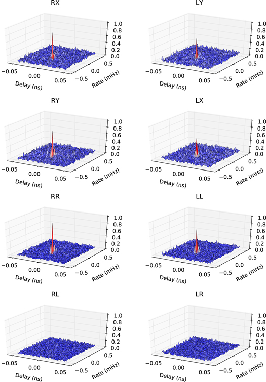
Figure 13. Delay-rate-fringe amplitude plots on a baseline between ALMA and the LMT during an APP CSV Band 6 observation of the quasar PKS J1512−0905 in 2016 April. Panels in the top two rows show the "mixed" linear (X and Y) and circular (R and L) polarization products. The bottom two rows show the data after processing with PolConvert to translate ALMA's linearly polarized data to circular (see Section 7). The boost in amplitude of the RR and LL fringes compared with RX and LY, and absence of signal in the cross hands of the converted data (RL and LR) demonstrate that the conversion is working nominally.
Download figure:
Standard image High-resolution image8. Performance of the Phasing System
8.1. Commissioning and Science Verification (CSV)
CSV for the APP was carried out over a two-year period from 2015 January to 2017 January. CSV activities used on-sky testing to validate the fully integrated components of the APS, including hardware, software, observing modes, recording modes, and correlation procedures. The tests that were carried out were designed to demonstrate that the APS met its formal design requirements, that the APS produces robust, scientifically valid data whose characteristics are well understood and documented, and that ALMA is capable of operating as a fully functional VLBI station. Presently these attributes continue to be checked by periodic regression testing of the APS. Details from the various APP CSV campaigns and supplementary test observations have been described in a series of ALMA Technical Notes (Matthews & Crew 2015a, 2015b, 2015c; Matthews et al. 2017).
8.2. Phasing Efficiency
As noted in Section 1, a perfectly phased array of  antennas is equivalent to a monolithic aperture with
  times the effective area of one of the individual elements,
  . However, in practice, any real phased array will suffer from efficiency losses (i.e., loss of effective collecting area) caused by a combination of factors. These losses may be collectively characterized in terms of a "phasing efficiency,"
  , where
  corresponds to perfect efficiency. Routine characterization of the phasing efficiency allows determining whether the system consistently meets theoretical expectations, and is crucial for enabling accurate absolute calibration of VLBI experiments. In addition, such a measure serves as a useful metric for comparing performance of the system under various conditions (e.g., different weather, array configurations, or observing frequencies).
The gain of an antenna may be defined as  where k is the Boltzmann constant (TMSIII). If the effective area of a single ALMA antenna is
  , then the gain of a phased array of
  such antennas may be written as:
  .
.
If we now correlate the phased sum signal  (Equation (1)) with the signal
  from another identical "comparison" antenna in the array that is not part of the phased sum, the resulting product can be written as

where ν is the observing frequency, t is the integration period, and  is the amplitude of the correlated signal (e.g., Condon & Ransom 2016). Because
  and
and  are both proportional to the electric field of the source being observed, multiplied by the gains of the sum antenna and comparison antenna, respectively, this implies that the amplitude term in Equation (6) is in turn proportional to
  . Thus for an ideal phased array, the correlated amplitude is expected to grow as the square root of the number of antennas used to construct the sum.
The phasing efficiency of the array,  , may then be parametrized as

where the  term in the denominator denotes the mean of the correlated amplitudes between each of the
  antennas used to form the phased sum and the unphased comparison antenna. (TelCal computes this ratio for a designated comparison antenna and provides the result within the ASDM file). Throughout the APP CSV, a variety of tests were used to gauge the overall efficiency of the APS empirically and to isolate the sources and magnitudes of various losses.
One means to characterize the efficiency of the phasing system is the execution of "step scan" sequences (Primiani et al. 2011) on bright, compact sources. During such an observation, antennas are sequentially added to, or subtracted from the phased array, permitting an evaluation of how correlated amplitude (and hence the phasing efficiency) scales with the number of antennas in the phased array. During a step scan test, one or more array antennas are designated as comparison antennas and are never phase-corrected or included in the phased sum.
Several step scan tests were performed using the APS during CSV campaigns. Results from one example are presented in Figure 14. These results are based on Band 6 observations of the quasar PKS J0522−3627 obtained with the APS on 2015 March 31. The weather conditions were relatively stable with PWV ∼ 1.3 mm. There were a total of 22 functioning 12-meter antennas in the array used for the test, three of which were designated as unphased comparison antennas. Baseline lengths ranged from 11 m to 313 m. During the course of a 10-minute observation, pairs of antennas were randomly added to or removed from the phased sum (hereafter designated "APP001," corresponding to the station identification of the phased sum in the ASDM file),19
with the maximum number of phased antennas being 19. The test was performed independently in the four basebands, resulting in different values of  in each quadrant at any given time. For clarity, we show here only the results for a single baseband/polarization combination (polarization XX in baseband 1, where the center frequency was 214.6 GHz) and for only one of the comparison antennas ("DA45"). Results for the other basebands and comparison antennas are comparable.
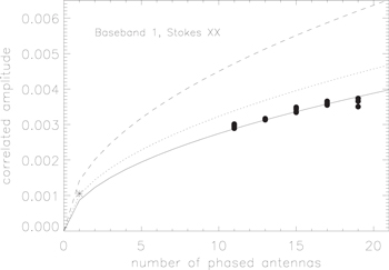
Figure 14. Results of a "step scan" phasing efficiency test of the APS performed on 2015 March 31 in Band 6. During a ∼10-minute observation, pairs of antennas were sequentially added to or removed from the phased array. The filled dots indicate correlated amplitude as a function of the number of phased antennas for baselines between the phased sum and an unphased comparison antenna. Each point is based on 16 s of data; results for only one of the eight baseband/polarization combinations are shown. The asterisk designates the correlated amplitude prior to phase-up of the array (i.e., it is comparable to a phased array of one antenna). The solid line shows a fit to the data (for  ) of the form
  where
where  is the number of phased antennas. The dotted line is the predicted result based on the
  measurement, while the dashed line shows the prediction for an ideal phased array. The results indicate that the amplitude generally increases with the number of phased antennas and that the overall phasing efficiency during the observation was ∼61%. See Section 8.2 for details.
Download figure:
Standard image High-resolution imageFigure 14 shows the correlated amplitude for the DA45–APP001 baseline as a function of the number of phased antennas for each 16 s subscan during the step scan test (closed dots). For each time interval, data from the 8 subbands within the baseband were averaged to yield a single amplitude value, and data from the first minute of data (during which the array was not fully phased) were excluded.
The solid line plotted on Figure 14 shows the result of a least squares fit to the measured amplitudes of the form  , where C is an arbitrary scaling factor. The correlated amplitude, A, is seen to follow the expected
  dependence for
  , but it is slightly lower than expected for
  . For comparison, the asterisk plotted on Figure 14 shows the correlated amplitude on the DA45-APP001 baseline prior to phase-up, i.e., effectively showing the amplitude for a phased array of one antenna. The dotted curve running through this latter point illustrates the correlated amplitudes that are predicted if this is adopted as a benchmark for behavior of the system. The actual measured values lie ∼15% below this curve. Finally, the dashed curve on Figure 14 plots the correlated amplitude expected for a perfectly phased array (
 ). We see that the measured amplitudes are ∼61% of those expected based on this idealized prediction. Unlike the values used to produce the dotted curve, those used to produce the dashed curve have not been processed by the summer mechanism. This therefore provides us a means of disentangling efficiency losses due to factors inherent to phase-correcting the antennas versus those inherent to the production of the phased sum signal itself.
Efficiency losses in the APS occur at different stages. First, imperfections in the phasing solutions themselves (as a consequence of tropospheric fluctuations, residual delay errors, source structure, and latency in the application of the phasing corrections) all increase the rms scatter,  , in the phases of the antennas used to form the phased sum. The decorrelation resulting from these fluctuations in turn produces a reduction in the correlated amplitude by a factor
  (e.g., Carilli et al. 1999). For the data set shown in Figure 14,
  rad (21°), hence
  . In general, the atmosphere dominates
  , hence efficiency will be worse at higher frequencies and in times of poor atmospheric stability. Nonetheless, in terms of these losses, the APS phasing engine routinely meets or exceeds its goal of 90% phasing efficiency as specified in the original functional requirements (see Section 3).
Second, a significant and unavoidable loss of phasing efficiency in the APS arises from the 2 bit quantization of the summed signal, which leads to an amplitude reduction of 12% (i.e.,  e.g., Kokkeler et al. 2001; Crew 2012). Third, additional smaller efficiency losses arise from discrete sum scaling errors (up to 5%) and the lack of optimized weighting of the contributions of the individual antenna signals to the sum. Ideally, one would want to weight the antenna contributions to the sum using either equal power or variance weighting (Moran 1989). However, the correlator circuit that receives the antenna data to be summed (provided by one of the so-called VLBI hooks; Baudry et al. 2012) does not have access to any additional data and has logic space only for a simple sum and not for additional weighting factors. Because the ALMA 12 m antennas are generally well matched (ALMA Partnership 2017, private communication), the weights should be approximately equal and this type of efficiency loss is not expected to exceed a few per cent.
Figure 15 shows results from another test of the APS, conducted on 2017 April 10 in Band 6 using an array of 37 phased 12 m antennas. The goal was to assess the phasing quality and stability as a function of time for all basebands and both polarizations. In this case, the number of phased antennas was kept fixed throughout. Four scans were obtained on the quasar PKS J1924−2914, during which the array was actively phased. Based on observations from the SMA,20
the 1 mm source flux density near the date of observation was 3.18 ± 0.16 Jy. The baseline lengths ranged from 14 m to 400 m and the PWV was ∼0.5 mm. The figure shows the rms scatter in the phases as a function of time for baselines between the phasing reference antenna and the antennas used to form the phased sum. At start-up, the array was completely unphased, as evidenced by the large phase scatter. Phase-up is achieved after approximately 20 s, after which the mean rms phase scatter is ∼10° across all of the four basebands, both polarizations, implying a decorrelation loss in amplitude of  .
.
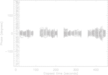
Figure 15. Phase as a function of time during a series of four Band 6 APS scans on the ∼3 Jy source PKS J1924−2914, conducted on 2017 April 10 using an array of 37 phased 12 m antennas. Phases are plotted for baselines between the phasing reference antenna and each of the individual antennas used to form the phased sum. Data for all four ALMA basebands, in both the XX and YY polarizations, are shown. Phase-up is achieved approximately 20 s into the first scan, after which the mean rms phase scatter is ∼10°.
Download figure:
Standard image High-resolution imageThese and other test data taken throughout CSV and subsequent regression testing show that under stable weather conditions, efficiency losses as a result of imperfections in the phasing solutions themselves are generally minimal. Note that during the second and fourth scans in the present example, the fast phasing loop was used in concert with the slow loop. We see that the rms scatter is ∼30% higher during those scans, confirming that these WVR-based corrections add noise when used under very stable weather conditions (see Section 5.2.3).
Importantly, the data shown in Figure 15 have been corrected by the APS phasing software, but they have not been processed by the summer, and are therefore not subject to the degradation in the signal caused by quantization errors and other subsequent losses. To assess these latter effects, we may examine the correlated amplitude on a baseline between the phased sum signal and an unphased comparison antenna,  , with respect to the correlated amplitude seen on a baseline between a comparison antenna and the phasing reference antenna
  . For a perfectly phased array subject to 2-bit quantization losses, the predicted ratio
  where
where  is the number of antennas in the phased sum. Instead, for the data set shown in Figure 15, we find
  , consistent with the results of the step scan test described above. Similar total efficiency values were also confirmed in subsequent VLBI observations (see Section 8.3).
Some portion of the APS efficiency loss can be attributed to the present treatment of baseband delays (see Section 5.2.4). This effect is expected to be of order a few per cent (Crew 2012). Additional factors contributing to an efficiency loss of ∼20% above the theoretical expectation remain a topic of ongoing investigation.
8.3. VLBI Fringes
The combined functionality of the various hardware components installed by the APP to enable VLBI operations at ALMA was successfully demonstrated for the first time on 2015 January 13 when a VLBI fringe on the quasar PKS J0522−3627 was detected at a frequency of 214.0 GHz (∼1.3 mm, i.e., Band 6) on a 2.1 km baseline between ALMA and the APEX telescope (Figure 16). Despite the short baseline, both stations used separate, independent frequency references, hence this constituted a true VLBI experiment. Although the ALMA station was operated as a multi-antenna array during this test, the array was unphased, and therefore the equivalent sensitivity was that of a single 12 m antenna.

Figure 16. VLBI fringe detection obtained on a 2.1 km baseline between ALMA and APEX on 2015 January 13 in Band 6 on the quasar PKS J0522−3627. Five seconds of data are shown. The data are of "mixed" polarization (ALMA's linear X polarization correlated against APEX's RCP data product). The clear peaks in the delay rate (red curve, top panel) and in the single-band delay (green curve, middle-left panel) and multi-band delay (blue curve, top panel) are consistent with the high S/N of the detection (∼68). The ALMA array was unphased during this observation, hence its sensitivity was equivalent to that of a single 12 m antenna. The center-right panel shows amplitude (blue) and phase (red), averaged over all baseband channels at a resolution of 100 kHz. The lower panel shows amplitude (blue) and phase (red) as a function of time for each of the thirty-two 51 MHz frequency channels. (The wings of the 62.5 MHz ALMA TFB channels were excluded). The fall-off in amplitude across the band is largely due to the characteristics of the APEX digital backend, which has better response at low frequencies.
Download figure:
Standard image High-resolution imageThe S/N expected for detection of a VLBI fringe between ALMA and another station may be expressed as

where we assume  is the efficiency of the APS (see Section 8.2),
  is a digital loss factor equal to 0.88 for 2 bit correlation of VLBI signals, S is the source flux density in Jy,
  is the number of polarizations,
  is the effective observing bandwidth, t is the integration time in seconds, and
  and
and  are the system equivalent flux densities (in Jy) of the two respective VLBI stations. The fringe shown in Figure 16 is based on 5 s of data, a single polarization (mixed linear–circular, R–X), and a usable bandwidth of 1632 MHz (32 channels of 51 MHz). Assuming a source flux density21
of ∼3.6 Jy and an SEFD of 3600 Jy for both the APEX and ALMA stations, the predicted S/N is
are the system equivalent flux densities (in Jy) of the two respective VLBI stations. The fringe shown in Figure 16 is based on 5 s of data, a single polarization (mixed linear–circular, R–X), and a usable bandwidth of 1632 MHz (32 channels of 51 MHz). Assuming a source flux density21
of ∼3.6 Jy and an SEFD of 3600 Jy for both the APEX and ALMA stations, the predicted S/N is  , while the observed S/N is 68 (note that these data are uncorrected for the use of mixed polarizations as described in Section 7). This implies
  , consistent with a nominal phasing efficiency after accounting for 2 bit quantization of the sum signal. Because the array was not summed in this case,
  is not subject to the additional efficiency losses described above for the
  case.
case.
Several subsequent VLBI fringe tests were performed with ALMA as a phased array, both in Band 3 and in Band 6 (Matthews & Crew 2015b, 2015c; Matthews et al. 2017). These tests included VLBI sessions of several hours duration during which a full suite of ALMA and VLBI-specific calibration sources were observed in order to permit end-to-end testing of PolConvert (see Section 7). One set of observations (experiment code BM452) was performed on 2016 July 10 in conjunction with the 8 stations from the National Radio Astronomy Observatory's22 VLBA that are equipped with 3 mm receivers.23 Two stations (North Liberty and Pie Town) were excluded from further analysis owing to poor weather.
An example of a fringe on the 6727 km baseline between a phased array of 11 ALMA antennas and the Fort Davis station of the VLBA is shown in Figure 17. The usable observing bandwidth was 204 MHz (four 51 MHz channels per polarization). The target source was the quasar PKS J0607−0834, which had a 3 mm flux density of ∼1 Jy near the time of the observations (see footnote 20). The peak source flux density is therefore comparable to the faintest VLBI science targets permitted during ALMA Cycles 4 and 5. However, the correlated flux density on the observed baseline is expected to be approximately four times lower (see Kovalev et al. 2005). Assuming an SEFD for the Fort Davis station of 3500 Jy, an SEFD for the phased ALMA array24
of 219 Jy, and an integration time of 238.4 s, the predicted S/N is ∼33 after accounting for known efficiency losses as described above (i.e.,  and
and  ) and applying PolConvert corrections (Section 7). Using an optimal segmentation time of ∼6 s for the data (to minimize decorrelation losses in the correlated amplitude), the measured S/N is 32.5, in excellent agreement with our previous characterizations of the system. This result confirms that the end-to-end phasing efficiency of the APS is routinely ∼61%, to within an uncertainty of a few per cent.
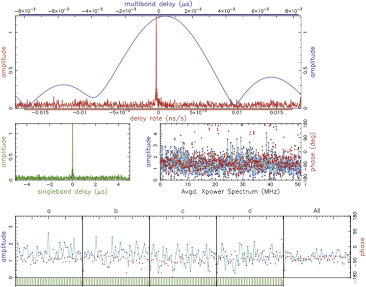
Figure 17. Fringe plot based on Band 3 scan of 238 s duration on the target source PKS J0607−0834 on a 6737 km baseline between ALMA and the Fort Davis VLBA station, obtained on 2016 July 10. The ALMA data have been converted from linear to circular polarization using PolConvert (Section 7); the resulting LL polarization is shown. The S/N of the fringe detection is ∼33. The panels are as described in Figure 16, with the exception that the Band 3 data shown here have a smaller total bandwidth (204 MHz, divided into four 51 MHz frequency channels, as shown in the lower panels).
Download figure:
Standard image High-resolution image
9. Future Enhancements
The implementation of the APS described herein, and offered during ALMA Cycles 4 and 5, provides the fundamental capabilities needed to perform VLBI with ALMA. However, extensions and expansions of the APS are currently being planned for future Cycles in order to further broaden and diversify the scientific applications of the phasing system.
One limitation of the current APS is the requirement that both the science target and the associated calibrators be point-like and sufficiently bright on intra-ALMA baselines to allow the phasing computations to be performed on the target itself. This restriction will be removed with the introduction of a "passive" phasing mode whereby phase-up is performed on a neighboring calibration source at an appropriate cadence. This will enable ALMA VLBI observations on significantly fainter targets, with the flux density limited by S/N considerations on a given VLBI baseline, rather than the need to phase up on the target of interest.
While the APS has so far been commissioned for use in ALMA Bands 3 and 6 only, there are no technical obstacles to using the system in other bands, provided that weather conditions are suitable for phasing. Implementation of the APS in the existing Band 7 (0.7 mm), the pending ALMA Band 1 (7 mm), and a possible future Band 2 (4 mm) is expected to be straightforward and require primarily a modest amount of on-sky testing to determine the optimal phasing parameters and the optimal range of array baseline lengths for use at these different wavebands. Band 7 operation of the APS is of particular interest for black hole studies, since the blurring effects of interstellar scattering will be minimized, thereby improving the ability to reconstruct images of the source (Johnson & Gwinn 2015; Johnson 2016). Use of the APS at still higher frequencies is also possible in principle, although it is unlikely to be advantageous owing to the increased atmospheric opacity at these wavelengths and the lack of other VLBI sites capable of commensurate operation. At the lower end of ALMA's frequency range of operation, Band 1 will provide frequency overlap with the Karl G. Jansky VLA, and offer an exquisitely sensitive baseline between ALMA and the phased VLA. Band 1 is also expected to be especially useful for pulsar searches (see below), as it provides a good trade-off between sensitivity and the minimization of interstellar scattering effects (e.g., Fish et al. 2013).
The ALMA frequency bands contain numerous astrophysically important spectral lines, and the observation of certain of these lines can benefit from the extraordinarily high sensitivity and/or angular resolution afforded by a phased ALMA (Fish et al. 2013, Tilanus et al. 2014). These include non-thermal molecular (maser) lines observable in emission (e.g., SiO, H2O, CH3OH, and HCN; Boboltz 2005; Wootten 2007) and weaker thermal lines detectable in absorption.
Targets for maser observations include evolved stars, young stellar objects, and the circumnuclear disks of galaxies, where maser studies with the highest achievable spatial resolution provide unique information on physical conditions, kinematics, and magnetic fields (e.g., Pérez-Sánchez & Vlemmings 2012; Richards 2012; Humphreys et al. 2016). Meanwhile, observations of absorption lines of HCN, HCO+, and other molecules with phased ALMA will be possible against background quasars in active galaxies, providing spatial information on the distribution of molecular gas (e.g., Carilli et al. 2000; Muller & Guélin 2008), enabling detailed studies of molecular and isotopic abundance ratios as a function of redshift (e.g., Muller et al. 2011), and providing constraints on possible variations of fundamental constants over cosmological times (e.g., Uzan 2011).
Enhancements to the APS to enable spectral line mode operation will include spectral window matching (to allow phase-up on a bright maser line), optimization of data rate management to allow higher spectral resolution in the ALMA standard interferometry data (they are currently spectral averaged by a factor of 8 to decrease data rates), and the exploration of modified correlation strategies for spectral line data sets. For example, the fringe-fitting of APS continuum data is currently done in the delay-fringe rate plane. But in the case of a spectral line where power is concentrated in the frequency domain, the delay function becomes broad and fringe-fitting may instead need to be performed in frequency-fringe rate space (Reid 1995). Further, the adopted correlation approach will need to be robust against the possibility of multiple peaks in the fringe rate resulting from atmospheric turbulence.
One other mode of APS operation that is expected to be of considerable interest to the community is use of the phased array as a "single dish" for pulsar searches in the mm domain. While pulsars are known to be relatively weak at ALMA frequencies, they are nevertheless expected to be detectable in ALMA bands (Torne et al. 2015; Mignani et al. 2017), and an important trade-off is that the effects from interstellar scattering become less severe at shorter wavelengths. High-frequency pulsar observations are therefore expected to allow identification of pulsars orbiting the Galactic center that could be used to provide novel tests of General Relativity (Cordes et al. 2004; Eatough et al. 2015; Psaltis et al. 2016). In addition, pulsar studies at mm wavelengths are expected to elucidate the processes that lead to observed changes in the spectral index above 30 GHz (e.g., Löhmer et al. 2008). Because pulsars are so faint at mm bands, a pulsar observing mode will depend on the passive phase-up mode described above, and will also benefit from implementation of a source modeler which features that ability to shift the array phasing center away from the pointing center.
10. Summary
The APP has led to the successful deployment of the hardware and software necessary to operate ALMA as a phased array and as the world's most sensitive mm VLBI station. These capabilities enable leveraging the enormous sensitivity of ALMA for science that requires extraordinary angular resolution, including studies of black hole physics on event horizon scales.
The current APS has been commissioned for use for continuum observations of bright ( Jy), compact targets in ALMA Band 3 (3 mm) and Band 6 (1.3 mm), and the first successful science observations using these capabilities were made in conjunction with the GMVA and EHT, respectively in 2017 April. Ongoing and future enhancements of the APS are expected to continue to expand and enhance the scientific applications of a phased ALMA in the coming years.
The APP gratefully acknowledges the support it received in wide-ranging areas from numerous individuals throughout the ALMA organization and at other institutes around the globe. It is nearly impossible to compile a comprehensive list of those who contributed to the APP's success, but among them are: H. Alarcon, J. Antongnini, J. Avarias, E. Barrios, U. Bach, A. Biggs, T. Beasley, L. Blackburn, J. Blanchard, R. Blundell, A. Bridger, W. Brisken, M. Caillat, R. Cappallo, J. Castillo, C. Chandler, M. Claussen, C. Coldwell, S. Corder, F. Cruzat, I. De Gregorio, A. Deller, B. Dent, M. Derome, P. Friberg, S. Fuica, E. Garcia, J. C. Gatica, J. Gil, C. Goddi, M. Gurwell, C. Jacques, D. Herrera, R. Hills, A. Hoffstadt, D. Hughes, J. Ibsen, H. Johnson, J. Kern, R. Kneissl, T. Krichbaum, R. Laing, C. Lonsdale, C. Lopez, R. Lucas, G. Marconi, L. Martinez-Conde, M. McKinnon, R. Lucas, R. Marson, S. Matsushita, A. Mioduszewski, G. Narayanan, L-Å. Nyman, J. Ogle, G. Ortiz-León, M. Parra, R. Porcas, R. Primiani, W. Randolph, A. Remijan, J. Reveco, A. Rogers, R. Rosen, N. Saez, A. Salinas, T. Sawada, J. Sepulveda, T-C. Shen, J. SooHoo, R. Soto, D. Sousa, T. Staig, M. Straight, S. Takahashi, C. Tapia, R. Tilanus, M. Titus, L. Vertatschitsch, E. Villard, J. Weintroub, N. Whyborn, K. Young, and A. Zensus. The APP was supported by a Major Research Instrumentation award from the National Science Foundation (award 1126433), an ALMA North American Development Augmentation award, ALMA North American Cycle 3 and Cycle 4 Study awards, a Toray Science and Technology Grant through the Toray Science Foundation of Japan, and a Grant-in-Aid for Scientific Research on Innovative Areas (25120007), provided by the Japan Society for the Promotion of Science and the Ministry of Education, Culture, Sports, Science and Technology (JSPS/MeXT). This work made use of data from NRAO projects BM434 and BM452.
Footnotes
- 16
- 17
- 18
The 7 m ACA dishes do not have WVR units installed and there are currently no plans to so equip them.
- 19
Strictly speaking, APP001 is a fictitious pad position corresponding to the array reference position.
- 20
The 1 mm flux density of J1924−2914 close to the date of observation was obtained from the SMA calibrator web site: http://sma1.sma.hawaii.edu/callist/callist.html. Measurements at this site are obtained with the SMA as part of an ongoing monitoring program (Gurwell et al. 2006). The measured source signal strengths are calibrated against known standards, typically solar system objects.
- 21
Ibid.
- 22
The National Radio Astronomy Observatory (NRAO) is a facility of the National Science Foundation operated under cooperative agreement by Associated Universities, Inc.
- 23
In 2016 October, operation of the VLBA was transferred from NRAO to the Long Baseline Observatory.
- 24
The estimated SEFD for phased ALMA during this test assumes 11 identical 12 m antennas, each with an aperture efficiency of 0.71 and a Band 3 system temperature of 70 K.