

Abstract
In the current manuscript, (4 + 1) dimensional Fokas nonlinear equation is considered to obtain traveling wave solutions. Three renowned analytical techniques, namely the generalized Kudryashov method (GKM), the modified extended tanh technique, exponential rational function method (ERFM) are applied to analyze the considered model. Distinct structures of solutions are successfully obtained. The graphical representation of the acquired results is displayed to demonstrate the behavior of dynamics of the nonlinear Fokas equation. Finally, the proposed equation is subjected to a sensitivity analysis.
Export citation and abstract BibTeX RIS
1. Introduction
Nonlinear partial differential equations (NPDEs) play a key role in physical and mathematical models. NPDEs define their ranges from fluid dynamics, gravitation, physical systems, mathematical models and they have been used in mathematic, for example, for solving the Poincaré as well as the Calabi conjectures. There are nearly no widespread procedures that perform for all problems, and generally, every separate model should be worked as an individual problem.
Solutions of PDEs had a supreme state in recent years. Often we can write solutions of NPDEs with some special solutions. The explicit solutions can be written by reducing given NPDE to equations of lower dimension and for this, we usually choose the way of converting it to ordinary differential equations. Reduction to ordinary differential equations is usually based on Lie symmetries and wave transformations. In literature recent years, lots of methods are given for solving NPDEs for example the tanh-coth strategy [1], the auxiliary equation technique [2, 3], modified simple equation technique [4], Bernoulli function methodology [5], the new extended direct algebraic technique [6], the sine-Gordon expansion technique [7, 8], Hirota bilinear technique [9], the simplest extended equation technique [10, 11], the F-expansion technique [12], He's semi-inverse technique [13], the sub-ODE technique [14], the (G'/G) -expansion technique [15], the generalized Kudryashov technique [16], and many more. The common point of all the methods mentioned here is to convert the PDEs to the ordinary differential equations (ODEs) with the help of wave transformations.
In this study, we are going to tackle the (4 + 1)-dimensional Fokas equation

Fokas [17] presented equation (1) by the expansion of Lax pairs of the integrable Davey-Stewartson (DS) and Kadomtsev-Petviashvili (KP) equations to some higher dimensional wave equations. The DS and KP equations have been used to investigate surface and interior waves in straits or channels of varying depth and width, as well as the evolution of a three-dimensional wave-packet on water of finite depth.
Lately, the proposed Fokas equation has been handled by different researchers. Lie point symmetries are given by Yang and Yan [18] and exact solutions are given by different technique, for instance the (G'/G) method [19], F-expansion scheme [20], and the modified tanh-coth methodology [21]. Tan et al . have founded a rogue wave solution and two homoclinic results of proposed equation [22]. Wang et al. used Bell polynomials to provide a bilinear form of the equation. Then they have obtained Riemann theta function soliton solutions and periodic solutions by utilizing the resulting bilinear formalism. [23]. Kumar et al. have employed the Lie group of transformation scheme to extract some exact outcomes of the considered equation [24]. Zang and Xia discovered the soliton solutions of the equation [25]. Khatri et al. have utilized three distinctive approaches to find traveling wave solutions of given equation [26]. Khatri et al. investigated a family of localized soliton and exact traveling solutions of this equation via distinct different methods, such as the Padés type transformation, the Jacobian-function method, triangle function approach or sine-cosine as well as the semi-inverse variational approach. The reported solutions are fractional solitons, localized soliton, Jacobi doubly periodic wave solutions [27]. Baskonus et al. investigated breaking soliton solutions of the equation via the sine-Gordon expansion method [28]. Mohammed, O.A employed the MSE method and the ESE strategy to get some fresh exact solutions [29].
2. Analysis of the proposed technique
To illustrate the concept of the steps of three distinct strategies, namely the GKM, the ERFM, and the modified extended tanh-function method will be described.
Think a model in NPDE form:

P involves U and its partial derivatives. Firstly, we utilize the common step to convert equation (2) to the nonlinear ODE. For this purpose, the following traveling wave transformation should be used [30, 31]:

and β, α, σ, γ,  are nonzero arbitrary constants with as a wave speed. Therefore, the following ODE is obtained:

here  .
.
2.1. Description of the GKM
The following are the next steps for GKM. Now, assume the initial solution of equation (4) as following [32, 33]:

here bj (j = 0, 1,...,M), ai (i = 0, 1,...,N), (aN ≠ 0, bM ≠ 0 ) are unknown coefficients to be found and R = R(ζ) is the solution of

which can be represented as

Now using principle of homogeneous balance, we find the values of M and N in equation (5). Lastly, we attain a polynomial of R by substituting the equations (5) and (6) into equation (4). The system of algebraic equations is obtained by equating all polynomial coefficients to zero. Find the values of unknown coefficients of bj (j = 0, 1,...,M), ai (i = 0, 1,...,N) using computer software. Finally, we derive the suggested equation's solitary wave solutions.
2.2. Key points of ERFM
The solution for equation (4) can be assumed as following [34] :

where aN
 are the unknown constants to be found. Using a homogeneous balance system, determine N in equation (4).
Putting equation (8) into equation (4) and separating all terms with the same order of en ζ (n = 0, 1, 2, ...) together, we make into the left-hand side of equation (4) another polynomial in en ζ . We next equate all of the polynomial's coefficients to zero, resulting in a set of algebraic equations for an . Finally, we solve the system equations to find the exact solutions for equation (2).
2.3. Modified extended tanh-function scheme
We will now discuss the modified extended tanh-function approach and offer the essential details. The explicit solution of equation (4) can be written by:

here a0, bi
and ai
 are arbitrary constants and they must be aN
≠ 0 or bN
≠ 0 at the same time. In equation (9)),
are arbitrary constants and they must be aN
≠ 0 or bN
≠ 0 at the same time. In equation (9)),  satisfies the Riccati equation in the following form:

here b is a constant. The known solutions of the Riccati equation are given as follows:
Hyperbolic solution: If b < 0, the following solution is given:

Trigonometric solution: If b > 0, the following solution is given:

Rational solution: If b = 0, the following solution is given:

Now put equation (9) and equation (10) in equation (4), we get a polynomials in  . Then equating each coefficient we obtain an over-determined set of equations for
  which on solving gives the values of unknown constants [35–37].
3. Applications of proposed schemes to Fokas equation
The GEM, ERFM, and modified extended tanh-function methods will be used to generate some exact solitary wave solutions of the Fokas equation in this section. For reducing equation (1) to ODE, we will use wave transformation equation (3). For this situation differentiations of U respect to independent variables are given by;

and similarly we obtain

Substituting equation (14) and equation (15) in equation (1), we get

If we integrate twice times equation (16), we obtain following reduced ODE

3.1. Exact solutions via the GEM
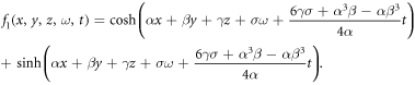
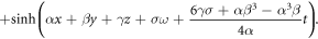
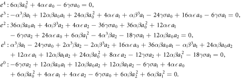
We found N = M + 1 to obtain the traveling wave solutions of the tackled model. Then, we may set N = 2 and M = 1. Therefore, we get

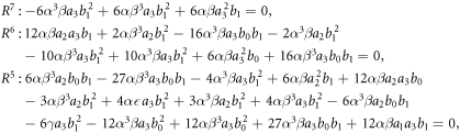
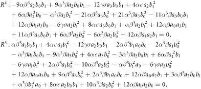
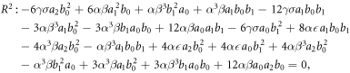
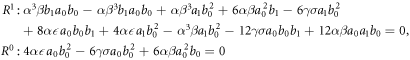
and substitute equation (18) into equation (17) and with equation (6). Equating each coefficient to zero, we get a system given below:
The following results are achieved by solving the above system:
Case 1:

Therefore, we subrogate these values to get the following solution:

where C1 is an arbitrary constant and
Case 2:

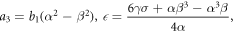
Therefore, we subrogate these values to get the following solution:

where

3.2. Exact solutions via the ERFM
According to balance number, the solution can be expressed as

Making use of equation (21) into the reduced equation (17) and collecting all terms with the same order of en
ζ
(n = 0, 1, 2, 3, 4) together, we obtain a polynomial of en
ζ
and, we equate each coefficient of this polynomial to zero yields a set of algebraic equations for an
, α, β, γ, σ and . Finally, we solve the equation system to construct a variety of exact solutions for equation(2).
Case 1:

Therefore, we subrogate these values to get the following solution:

Case 2:

Therefore, we subrogate these values to get the following solution:

3.3. Exact solutions via the modified extended tanh-function method
We said in the previous subsection that balancing is 2. Then the solution can be considered in the form below

If we substitute equation (24) into the equation (17), we obtain the following system.


If we solve above system, we get six cases.
Case 1:

Then, exact solutions are given in the following form.
When b < 0,

When b > 0,

When b = 0,

where 
Case 2:

When b < 0,

When b > 0,

When b = 0, the same solution equation (27) is obtained.
where 
Case 3:

When b < 0,

When b > 0,

When b = 0, the same solution equation (27) is obtained.
where 
Case 4:

When b < 0,

When b > 0,

When b = 0, the same solution equation (27) is obtained.
where 
Case 5:

When b < 0,

When b > 0,

When b = 0, we obtain zero solution.
where 
Case 6:

When b < 0,

When b > 0,

When b = 0, we obtain zero solution.
where 
4. Sensitive analysis
This section explains the suggested system's sensitive behavior. The effects of uncertainty on the output of model parameters can be quantified through sensitivity analysis. Sensitivity analysis investigates how different values of an independent variable affect a certain dependent variable under a set of assumptions. The main goal of this investigation is to precisely measure the output perturbation caused by the input fluctuation. In this section, where results are presented utilizing a range of parametric values, the analysis may be noted by studying how little changes in input can result in a significant change in the conclusion. The following figure 8 is a detailed study of the current system.
5. Conclusions
In this manuscript, three different approaches, the GKM, ERFM, modified extended tanh-function method have been applied to acquire new soliton-type solutions of the proposed (4 + 1)-dimensional Fokas equation. Methods are useful for given equation. We obtained different solutions from each other. Solutions are given by hyperbolic,trigonometrics,rational function solutions. We have seen that the methods discussed in our study are applicable to the Fokas equation. Lee and Sakthiver in [21] used modified tanh-coth method for obtaining exact solution of Fokas equation. Our results are different from their results. If we implement the extended tanh-function method [38] to given model, we get the same solutions with case 1 and case 2. Finally, the dynamical system was explored to determine its sensitivity and the behavior was visualized using initial conditions.
6. Discussion
In this study, we have adopted three distinct techniques to obtain the traveling wave solutions of the (4 + 1)-dimensional nonlinear Fokas equation. All the obtained solutions are different from each other and they consist of different variables. We can state the following comparison statements for the used techniques in this manuscript. For the GEM and modified extended tanh-function methods, we used auxiliary equations for the solutions of the dealt equation, which are different from each other. For the ERFM, we don't use an auxiliary equation. We have also given a sensitive analysis of the system to show that how much the system is sensitive on the behalf of initial conditions. The figures in this section highlight the changes when we change the initial conditions.
The graphical representations are visualized to display the spatial-temporal distribution of the obtained traveling wave solutions. We gave 3D graphs for some solutions with figures. 1–7. The figure 1 solution for U1(x, y, z, ω, t) when C1 = 1, α = 1, β = 2, the figure 3 solution for U3(x, y, z, ω, t) when β = 2, α = 1, the figure 4 solution for U4(x, y, z, ω, t) when α = 1, β = 2 are bright soliton solutions. We see that the figure 2 solution for U2(x, y, z, ω, t) when C1 = 1, β = 1, α = 2 is dark soliton solution. In the figure 5 solution for U5(x, y, z, ω, t) when α = 1, β = 2, b = − 2, we see that the solution is bell type soliton solution. The figure 6 solution for U6(x, y, z, ω, t) when b = 2, β = 2, α = 1 is periodic wave solution and finally the figure 7 solution for U7(x, y, z, ω, t) when β = 2, α = 1, b = 0 is kinky periodic wave solution.

Figure 1. The figure solution for U1(x, y, z, ω, t) when C1 = 1, α = 1, β = 2.
Download figure:
Standard image High-resolution image
Figure 2. The figure solution for U2(x, y, z, ω, t) when C1 = 1, α = 2, β = 1.
Download figure:
Standard image High-resolution image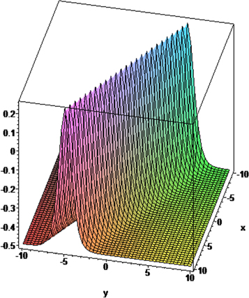
Figure 3. The figure solution for U3(x, y, z, ω, t) when β = 2, α = 1.
Download figure:
Standard image High-resolution image
Figure 4. The figure solution for U4(x, y, z, ω, t) when β = 2, α = 1.
Download figure:
Standard image High-resolution image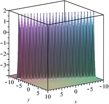
Figure 5. The figure solution for U5(x, y, z, ω, t) when b = − 2, α = 1, β = 2.
Download figure:
Standard image High-resolution image
Figure 6. The figure solution for U6(x, y, z, ω, t) when b = 2, α = 1, β = 2.
Download figure:
Standard image High-resolution image
Figure 7. The figure solution for U7(x, y, z, ω, t) when b = 0, α = 1, β = 2.
Download figure:
Standard image High-resolution image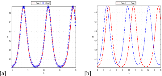
Figure 8. (a) shows the sensitivity of the system letting the initial conditions (U, V) = (0.02, 0.015) and (U, V) = (0.02, 0.01) with γ = α = − 1, σ = 1, β = 1.5 and ε = 0.5. It is essential to note that overlapping between curves can be seen. (b) takes the conditions (U, V) = (0.02, 0.015) and (U, V) = (0.05, 0.035) respectively.
Download figure:
Standard image High-resolution image
Data availability statement
The data that support the findings of this study are available upon reasonable request from the authors.
Funding
No funding was received for conducting this study.
Conflicts of interest
Authors declare there is no conflict of interests regarding the publication of this paper.
Availability of data and material
All data generated or analyzed during this study are included in this published article.