


Abstract
The problem of characterizing classical and quantum correlations in networks is considered. Contrary to the usual Bell scenario, where distant observers share a physical system emitted by one common source, a network features several independent sources, each distributing a physical system to a subset of observers. In the quantum setting, the observers can perform joint measurements on initially independent systems, which may lead to strong correlations across the whole network. In this work, we introduce a technique to systematically map a Bell inequality to a family of Bell-type inequalities bounding classical correlations on networks in a star-configuration. Also, we show that whenever a given Bell inequality can be violated by some entangled state ρ, then all the corresponding network inequalities can be violated by considering many copies of ρ distributed in the star network. The relevance of these ideas is illustrated by applying our method to a specific multi-setting Bell inequality. We derive the corresponding network inequalities, and study their quantum violations.
Export citation and abstract BibTeX RIS

Original content from this work may be used under the terms of the Creative Commons Attribution 3.0 licence. Any further distribution of this work must maintain attribution to the author(s) and the title of the work, journal citation and DOI.
1. Introduction
Bell inequalities bound the strength of correlations between the outcomes of measurements performed by distant observers who share a physical system under the assumption of Bell-like locality. Famously, quantum theory predicts correlations, mediated by entangled states, that violate Bell inequalities [1]. Such nonlocal quantum correlations are central for many quantum information tasks as well as foundational challenges [2]. Classical and quantum correlations in the standard Bell scenario, i.e., where distant observers share a physical system produced by a single common source, have been intensively studied and are by now relatively well understood.
In comparison, only very little is known about classical and quantum correlations in networks. The latter are generalizations of the Bell scenario to more sophisticated configurations featuring several independent sources. Each source distributes a physical system to a subset of the distant observers. In the classical setting, each physical system is represented by a classical random variable. Importantly, random variables from different source are assumed to be independent. In the quantum setting, each source can produce an entangled quantum state. Moreover, each observer can perform joint (or entangled) measurements on systems coming from different sources—e.g., as in entanglement swapping [3]—thus potentially creating strong correlations across the entire network. Understanding the strength of quantum correlations in networks is a challenging problem, but of clear foundational interest. In addition, practical developments of quantum networks make these questions timely, see e.g. [4, 5].
One of the main hurdles for solving the above problem, is to first characterize classical correlations in networks. This turns out to be a challenging problem. Due to the assumption that the sources are independent, the set of classical correlations does not form a convex set anymore, as it is the case in the usual Bell scenario. Therefore, in order to efficiently characterize classical correlations, one should now derive nonlinear Bell-type inequalities. Only a handful of these inequalities have been derived so far. First works derived inequalities for the simplest network of entanglement swapping [6, 7], for which experimental violations were recently reported [8, 9]. Then inequalities for networks in the star-configuration were presented [10]. There exists also methods for deriving nontrivial Bell-type inequalities for other classes of networks [11–13]. Entropic Bell inequalities has also been derived for several networks [14], but are usually not very efficient at capturing classical correlations. Furthermore, another approach to study correlations in networks is from the point of view of Bayesian inference [15–21].
In this work we aim to establish a direct link between the well-developed machinery of Bell inequalities, and the much less developed study of Bell-type inequalities for networks. Here, we focus on star-networks. We introduce a technique that allows one to map any full-correlation two-outcome bipartite Bell inequality into a family of Bell-type inequalities for star-networks (henceforth referred to as star inequalities). Specifically, starting from any such Bell inequality, we construct star inequalities for any possible star-network, which efficiently capture classical correlations. As a special case, this allows us to recover previously derived star inequalities [7, 10] by starting from the CHSH Bell inequality [22]. In general, our approach has three appealing features. First, the star inequalities we derive can have any number of settings for all observers. Second, our star inequalities efficiently capture the non-convex set of classical correlations, as there exist probability distributions violating our inequalities that would not violate any standard Bell inequality. Third, their quantum violations can be directly related to the quantum violation of the initial Bell inequality. More precisely, we show that whenever an entangled state ρ violates a Bell inequality, then all the corresponding star inequalities can be violated by placing many copies of ρ in the star-network. Conversely, we show that certain quantum correlations in star-networks can be used to infer bounds on independent Bell tests. Finally, we illustrate the relevance of this method by an explicit example in which we start from a Bell inequality with more than two settings and construct the mapping to a particular star inequality and study its violation in the simplest network of entanglement swapping.
2. Star networks and N-locality
Star-networks are a class of networks parametrized by the number of independent sources N. The network thus involves  observers: N so-called edge observers each of whom independently shares a state with one common central observer called the node observer. See figure 1 for an illustration.
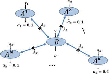
Figure 1. Star-network with a node observer B and N edge observers  each independently sharing a bipartite physical system with the node observer.
Download figure:
Standard image High-resolution imageThe k'th edge observer performs a measurement labeled by xk (chosen among a finite set) returning a binary outcome ak. Depending on the context, to be consistent with previous work, we label it either  (sections 4, 6 and 7) or
  (as soon as correlators are involved). The node observer performs a measurement labeled by y returning an outcome b. The resulting statistics is given by a conditional probability distribution of the outcomes of all observers given their inputs. This probability distribution is called N-local if it admits the following form:

where we have used the short-hand notation  . In an N-local model (which is the analogue of a local model in the Bell scenario), each independent source emits a random variable
  which is shared between a subset of the observers. In particular, for the star network, each edge observer shares a
  (possibly encoding an unlimited amount of shared randomness) with the node observer. Importantly, the sources are assumed to be independent from each other, and thus the variables
  are uncorrelated. Since the node observer holds
  , he can create correlations among all observers. Notice that if N = 1 we recover the definition of classical correlations in the Bell scenario. If the probability distribution cannot be written on the above form, it is said to be non N-local. Inequalities bounding the strength of N-local correlations arising in a star network are called star inequalities.
3. Mapping Bell inequalities to star inequalities
Consider a bipartite Bell scenario, where two observers Alice and Bob each perform one of nA respectively nB measurements on a shared physical system. Each measurement returns a binary outcome, now denoted  for convenience, where x and y indicate the choice of measurement of Alice and Bob respectively. Any full-correlation Bell inequality can be written

where Myx are real numbers, and C is the local bound. Note that  denotes the expectation value of the product of the outcomes of Alice and Bob. In equation (2) the superscript bs only serves as a label for the Bell scenario. Importantly, one can fully characterize the Bell inequality by specifying the matrix
  , from which the local bound C can be computed as follows. It is sufficient to consider deterministic strategies of Alice and Bob, due to the fact that the set of local correlations in the Bell scenario is a polytope [2]. Hence, we can write

where  . From now on, we use this notation for a linear transformation M of Alice's set of correlators. To maximize SbsM, we choose
  , which allows us to write the classical bound as


We now show how any Bell inequality of the form (2) can be mapped into a family of star inequalities for star-networks with N sources.
Theorem 3.1. For any full-correlation Bell inequality represented by the matrix  with corresponding classical bound
  , we can associate star inequalities as follows:

where

and

for some boolean functions  . Thus, specifying the real-valued matrix
  and the functions
  returns a specific star inequality for a star-network with
  sources.
The proof is rather technical hence we defer it to appendix A, where we prove a generalized version of the above theorem in which the star inequality is obtained as a mapping of up to N different full-correlation Bell inequalities, each characterized by a real-valued matrix  for
for  . The only restriction on the N Bell inequalities is that one observer (the one that by theorem 3.1 is mapped to the node observer) in each inequality chooses between the same number of measurements. For sake of simplicity, we have in the above taken all these N Bell inequalities to be represented by the same matrix, namely M. Furthermore, we note that generalizations of our theorem to networks of the type studied in [23], in which each source emits a multiparty physical system, are possible1
.
. The only restriction on the N Bell inequalities is that one observer (the one that by theorem 3.1 is mapped to the node observer) in each inequality chooses between the same number of measurements. For sake of simplicity, we have in the above taken all these N Bell inequalities to be represented by the same matrix, namely M. Furthermore, we note that generalizations of our theorem to networks of the type studied in [23], in which each source emits a multiparty physical system, are possible1
.
An important feature of the star inequalities generated via the above construction is that they give a better characterization of the N-local set compared to standard Bell inequalities. That is, there exist certain probability distributions that are not N-local (as witnessed by the violation of some of our inequalities) that are nevertheless local in the usual Bell scenario (i.e. 1-local), and thus cannot violate any standard Bell inequality. This is made explicit in the next section.
4. Recovering the inequalities of [7, 10]
As an example of our technique, consider the CHSH inquality [22] which corresponds to the 2 × 2 matrix  for x, y = 0, 1. The local bound (4) is straightforwardly evaluated to C = 1. Choosing a star-network with two sources (N = 2), and letting the node observer perform one complete two-qubit measurement with outcomes
  , we can define
  and immediately recover the inequality of [7]:

where I1 and I2 are defined via equation (7). Also, by letting the node observer have two measurement settings ( ), one associated to I1 and one associated to I2, returning an output bit
  , we recover the other inequality of [7] with
  (this example will be studied in more detail in appendix B3). Similar mappings of the CHSH inequality also return the star inequalities of [10] valid for an arbitrary number of sources:

In this scenario, all observers have two settings and two outcomes, and  . For N = 1 this reduces to the CHSH inequality.
Importantly, the above star inequalities are nonlinear, and thus give a better characterization of the N-local set compared to standard (linear) Bell inequalities. In particular, there exist quantum correlations admitting a local description (hence not violating any standard Bell inequality) that nevertheless violate these star inequalities [7, 10].
5. Optimal classical strategies and tightness
We now demonstrate a property of optimal N-local strategies regarding our star inequalities. We show that for any star inequality obtained from theorem 3.1, any N-local strategy achieving  with given values
  can be replaced with another N-local strategy achieving the same
  in which the node observer B acts trivially i.e. gives a deterministic output depending on the input. Moreover, this is achieved with the same strategy for each edge observer Ak. More precisely, we have the following:
Proposition 5.1. For any  -local strategy
  reaching the the
  -local bound in equation (6) with
  , there is a reduced strategy
  such as:
- 1.The node observer B has a deterministic output:
 is independent from and only depends on . We note it : this is the deterministic output of B for input . Thus each source of randomness can be considered as local and held by the edge observer .
 - 2.Each edge observer chooses her output according to the same strategy: the functions are independent from (then we write ).
- 3.The quantities Ii remain unchanged:.


This proposition is proven in appendix B, in which we also illustrate it by applying it to a particular example.
Another question is whether any set  saturating the inequality (6) can be obtained by an N-local strategy. We see in appendix C that this is not the case and give a way to find and enumerate all the sets
  satisfying this property.
So far, we have shown how the limitations of classical correlations in the Bell scenario can be mapped to analog limitations in networks. Next, we explore if an analogous statement can be made for quantum correlations.
6. Quantum violations
We shall relate the quantum violation of the initial Bell inequality to the quantum violation of the corresponding star inequalities. Specifically, we will see that for any state ρ violating the initial Bell inequality, taking a sufficient number of copies of ρ distributed in the network will lead to violation of the corresponding star inequality. Also, the robustness to white noise of every quantum state violating a Bell inequality (2), is the same as that of N copies of the same state violating a star inequality.
Consider a Bell scenario where Alice and Bob share an entangled state ρ and perform nA and respectively nB binary local measurements represented by observables  and
and  . This leads to violation of some full-correlation Bell inequality, i.e. achieving
  . Then we obtain a quantum strategy for violating the corresponding star inequalities as follows.
Let the node observer in the star-network perform nB different measurements. Each one is represented by an observable which is simply the N-fold tensor product of the measurements performed by Bob in the Bell scenario:  , and let all the edge observers perform the same nA measurements as Alice in the Bell scenario:
  . Finally, let all N sources emit the same bipartite state ρ as in the Bell scenario. This causes the factorization
  which implies

Inserting this into equation (6) we recover  . We conclude that

Note the generality of the above statement, which holds true for any full-correlation Bell inequality and all its corresponding star inequalities (in particular for all possible choices of functions fi(b)). Moreover, the statement holds for an entangled state ρ of arbitrary Hilbert space dimension.
The case of CHSH Bell inequality deserves to be discussed. The above statement implies that any entangled state violating CHSH will violate all its corresponding star inequalities when enough copies are distributed in the network. In particular, this is case for any pure entangled bipartite state [24], and more generally for any two-qubit state detected by the Horodecki criterion [25] (necessary for CHSH violation). Note that the latter statement was recently derived in [26] for the case N = 2, however, with the important difference that there the node observer performed a Bell state measurement whereas in our case we consider product measurements.
Conversely, if the node observer performs some product measurement, i.e., a measurement of the form  , with otherwise arbitrary choices of measurements for all edge observers and N arbitrary states distributed in the network, then the achieved value of Snet is upper bounded by the geometric average of Sbs as obtained in N independent Bell tests. Due to the separability of
  , we have
  . Inserting this into equation (6) we find

To obtain the upper bound, we have used lemma A.1 stated in appendix A, which may be regarded as a generalization of the Cauchy–Schwarz inequality. The expression on the right-hand-side of equation (13) is the geometric average of  as obtained in N independent Bell tests M, each performed on the state
  with settings of Alice and Bob determined by the settings used to achieve Snet in the star-network. This upper bound coincides with Snet only when all N Bell tests yield the same value
  .
.
So far, we have only considered product measurements of the node observer, which were sufficient to map quantum strategies in Bell inequalities to analog strategies in networks. Next, we consider an explicit example of a multisetting Bell inequality from which we construct a star inequality for N = 2 and study the quantum violations using product and joint measurements.
7. Example: quantum correlations from entanglement swapping
We consider the full-correlation Bell inequality presented in [27] 2 . It is represented by the following matrix;

We can calculate the classical bound using equation (4), and write the associated Bell inequality, in which Alice has four settings and Bob has three settings, as follows:

The maximal quantum violation of this inequality is given by  , obtained with a maximally entangled two-qubit state
  . Alice's measurements are characterized by Bloch vectors forming the vertices of a tetrahedron on the Bloch sphere:

Bob's measurements are simply given by the three Pauli matrices  , and
, and  . If we consider the mixture of
  with white noise, i.e. a Werner state of the form

the inequality can be violated whenever  . Note that a sufficiently high violation of this inequality implies that the measurements settings do not lie in a plane of the Bloch sphere, i.e. they feature complex phases [28].
Next, we obtain a particular star inequality for N = 2 in which we let each edge observer perform one of four measurements  , whereas the node observer performs a single measurement (i.e. no input y) with four possible outcomes
  . This is illustrated in figure 2. To this end, we apply our theorem 1. We define three quantities

where

We choose the functions fi(b) for  as:
as:  . Hence, our star inequality reads


Figure 2. The node observer performs a single measurement with four possible outcomes and the two edge observers each perform one of four measurements with binary outcomes.
Download figure:
Standard image High-resolution imageNext we discuss quantum violations. Both sources in the network emit the Bell state  . The two edge observers perform the four tetrahedron measurements given in equation (16). The node observer performs the Bell state measurement projecting her two systems onto the basis of maximally entangled two-qubit states:
  . Such a Bell state measurement typically causes the joint state of the subsystems of the two edge observers to become entangled, with its exact form depending on the outcome of the node observer. The resulting expectation values are

where  . This leads to
  which inserted into equation (20) returns
  . Hence, quantum correlations generated in an entanglement swapping scenario violate the considered star inequality. If both sources are noisy and each emits a Werner state
  , then one can violate the inequality (20) whenever
  . This coincides with the critical noise level of the Bell inequality in equation (14).
Furthermore, note that we can with minor modification re-cast our inequality (20) so that the node observer performs three different measurements, each with a binary outcome b. In this scenario, one can again obtain the quantum violation  . Note in this case the node observer uses three product measurements of the form
  , i.e. a product of Pauli matrices. It turns out that these three measurements are compatible (they commute). They can thus be measured jointly, which is done via the Bell state measurement.
Finally, we point out that we can swap the roles of Alice and Bob in the Bell inequality equation (15) so that when mapped to the star inequality, the node observer has four settings and the edge observers each have three settings. That inequality reads

where  , where
  . By letting the node observer perform products of the measurements in equation (16) and the edge observers perform the Pauli measurements
  for
for  , we again find a violation
  , for which the critical visibility again is
  .
.
8. Conclusions
Our main result is a method for systematically mapping any multi-setting full-correlation Bell inequality into a family of inequalities bounding the strength of classical correlations in star networks. This construction also allows us to show that quantum strategies for Bell inequalities can be mapped into analogous quantum strategies on star-networks. Specifically, for any entangled state ρ violating the initial Bell inequality, it follows that by taking enough copies of ρ in the star network one obtains a quantum violation of the corresponding star inequalities. Finally, we considered an explicit scenario involving more than two settings and show that quantum correlations in an entanglement swapping experiment can violate our inequalities.
To conclude, we mention some open problems: (1) Can our technique be extended to also include mappings of Bell inequalities with marginals, i.e. not only full-correlation terms as in equation (2). Whether the technique can be adapted to full-correlation Bell inequalities with more than two outputs (see e.g. [29]) is also relevant. (2) In particular, our technique allows us to explore quantum correlations in entanglement swapping experiments with many settings. Exploring the ability of these correlations to violate the inequalities would be of interest. (3) How can one extend our technique to involve networks that are not of the star configuration? (4) Can one construct star inequalities analogous to the one in equation (22) in which the node observer performs a single joint measurement with four outcomes? To what extent can quantum theory violate these inequalities? (5) It appears, after considering several particular examples, that all star inequalities derived by the presented technique cannot outperform the original Bell inequality in terms of noise tolerance when mixed with the maximally mixed state. Is this the case for any joint measurement? Or on the contrary, can one find an example where the use of an adequate joint measurements allows for activation of nonlocality. That is, while the entangled state ρ would not violate the initial Bell inequality, many copies of ρ distributed in the network would lead to violation of the star inequality. While such activation phenomena are proven to exist even when considering the standard definition of Bell locality [30, 31], we expect that the effect of activation should become much stronger when considering N-locality.
Acknowledgments
This work was supported by the Swiss national science foundation (SNSF 200021-149109 and Starting Grant DIAQ and QSIT), and the European Research Council (ERC-AG MEC).
Appendix A.: Proof of main theorem
In this appendix we prove a generalized version of theorem 3.1, in which the star inequality is obtained as mapping of up to N different full-correlation Bell inequalities in all of which at least one observer has the same number of settings. However, we first state a useful lemma that was presented and proven in [10]:
Lemma A.1. Let  be non-negative real numbers and let
  be integers. Then, the following relation holds:

with equality if and only if  .
.
Equipped with this lemma, we state and prove our main theorem.
Theorem A.2. Consider any set of  full-correlation Bell inequalities such that in every Bell scenario Bob has
  measurement settings, whereas in the k'th Bell scenario Alice has
  measurement settings. The k'th Bell inequality is represent by the matrix
  with associated classical bound
  . To every set of such matrices,
  , we can associate a family of star inequalities as follows:

where


and

for some boolean functions  . Thus, specifying the real-valued matrices
  and the functions
  returns specific star inequality for the star-network with
  sources.
Proof. Impose a classical model (1) on the probabilities in the quantities Ii defined in equation (7). This gives

Applying an absolute value to both sides allows for the following upper bound;

Each integral in the product series is a non-negative number. Hence, the quantity  can be upper bounded by a geometric average of such integrals. Applying the lemma A.1 to put an upper bound Snet, which is a sum of such quantities, we obtain the following:

Remember that each correlator of Alice obeys  and hence, using the classical bound (4) of the Bell inequality associated to
  to substitute in the integrand, we find

Using that  , we obtain the final result

■
Remark. By choosing all the N Bell inequalities to be the same, i.e. setting  , we obtain the special case of this theorem considered in the main text.
Appendix B.: Redundancy of node observer in classical strategies
Here we prove proposition 5.1 and illustrate it on a simple example.
Proof. Let us consider that we already have a strategy  reaching the bound in equation (6) with given Ii.
  is defined by the correlators of each edge observer Ak (resp. node observer B) given
  (resp.
  ) i.e.
  (resp.
  ). These correlators are such as:


As we have equality in equation (6), going back in the proof of theorem 3.1,  must be such as equation (A7) and equation (A8) are equalities. From the equality condition of equation (A7), we will deduce a
  satisfying condition 1. and 2. of the proposition. We then improve it in a strategy
  satisfying 3., using the equality condition of equation (A8).
Equation (A7) is the continuous triangle inequality. As we have equality, for any i, the integrand  must be of constant sign (the weights qk are positive). Then, any change in the sign of some
  at a specific
  must be compensated by a change of the sign of
  at the same
  , whatever are the other λj's (see figure 3). As
  , we have that:

where  depends on the sign of
  .
.
We now can define the new strategy  :
:

Through the transformation induced by M, this corresponds to corresponding  .
.
As  , the new
  corresponding to strategy
  are equal to the Ii corresponding to strategy
  . Then 1. and 2. of 5.1 are satisfied by
  . Moreover, we have:

We now use the equality condition of lemma A.1 and equation (A8) to prove 3. It is a convexity inequality which now reads:

were here the inequality is an equality. The condition for the convexity inequality in lemma A.1 to be an equality is that  is independent of k: we have here that for each
  . Replacing each the strategy and local random source of each edge observer Ak by a copy of the first edge observer A1 strategy and random source in
  (we then leave the exponent k), we may only change the sign of Ii. This can be compensate by an appropriate choice of
  . Then, we do not change 1. and 2. and obtain 3., with:

■

Figure 3. Illustration of the argument for two edge observers. As  is of constant sign (here positive) and
  , the sign of
  and
and  totally determine
  , which is of the form given by (B3).
Download figure:
Standard image High-resolution imageTo illustrate the proposition, let us recall the proof of the tightness of an inequality (already introduced in section 4) presented in [7], for a star network with N edges, two inputs and two outputs for each observer. As illustrated in the section Recovering the inequalities of ([7, 10]), the inequality can be seen as a direct application of theorem 3.1, taking a matrix M corresponding to a renormalized CHSH inequalitie,  . Then
  and
and  and
and  in equation (B2) is (I, J) in [7], with an inequality which writes:

The authors obtained the classical bound (restricting to  ) for each possible
  with the following strategy:


where the  are uniform shared variables between each of the edge observer and the node observer and the
  (
( with probability r) are sources of local randomness for each edge observer. We see here, as shown by the proposition, that all edge observer have the same strategy and that the node observer's strategy factorizes in
  with
with  . Then, as suggested by the proposition, defining:


we see that the Ii are unchanged by the transformation, and obtain a reduced strategy in which all the conditions of the proposition are satisfied. The proposition states that such a transformation is always possible.
Appendix C.: Partial tightness of star inequalities
We now study the tightness of the bound in equation (4):

In the following, using proposition 5.1, we find all the sets of  which are reachable by N-local strategies and saturate (C1).
We start by enumerating all the possible deterministic strategies for each edge observer:  for
for  . For each one, we note
  the vector obtained after transformation of X by M:

Suppose that a given set  satisfying condition (C1) can be obtained with an N-local strategy. Then, by proposition 5.1, we can suppose that it is obtained with a strategy in which the node observer B has deterministic strategy
  and all edge observers Ak play the same strategy (we then leave the exponent k) based on a shared random variable. Hence,

As A has only  possible deterministic strategies, there exists probabilities
  such that the strategy of each A is 'play deterministic strategy Xr with probability pr'.Then:

We then have:

where the inequalities are equalities, which implies:
-
i.e. for any i, the sign of all such as is the same (but may differ from one i to the other).
-
such as


Then, this proves that any distribution of  such as (C1) can be generated from the following method:
- 1.Enumerate all the possible
- 2.Keep the one such as.
- 3.Sort them in different sets Sν of size sν, each Sν containing where is constant over r (but may differ depending on i).
- 4.


