


Abstract
The actin cytoskeleton and its response to external chemical stimuli is fundamental to the mechano-biology of eukaryotic cells and their functions. One of the key players that governs the dynamics of the actin network is the motor protein myosin II. Based on a phase space embedding we have identified from experiments three phases in the cytoskeletal dynamics of starved Dictyostelium discoideum in response to a precisely controlled chemotactic stimulation. In the first two phases the dynamics of actin and myosin II in the cortex is uncoupled, while in the third phase the time scale for the recovery of cortical actin is determined by the myosin II dynamics. We report a theoretical model that captures the experimental observations quantitatively. The model predicts an increase in the optimal response time of actin with decreasing myosin II-actin coupling strength highlighting the role of myosin II in the robust control of cell contraction.
Export citation and abstract BibTeX RIS

Original content from this work may be used under the terms of the Creative Commons Attribution 3.0 licence. Any further distribution of this work must maintain attribution to the author(s) and the title of the work, journal citation and DOI.
1. Introduction
Mechanical stability, shape, and locomotion of eukaryotic cells, as well as numerous internal cellular processes critically depend on the dynamics and self-organization of the actin cytoskeleton [1–3]. Besides actin, the motor protein myosin II is of great importance in cell motility, cytokinesis, and development [4, 5]. In this work, we mainly focused on axenic, aggregation competent cells of the social amoeba Dictyostelium discoideum and the relevance of myosin II upon global chemoattractant stimulation. Myosin II is involved in numerous processes where contractility and actin-crosslinking functions are relevant, thus as front-back polarization, for example via the MTOC orientation and nuclear positioning, apical constriction and thus epithelial apico-basal cell polarity, uropod retraction and adhesion dissolution, leading edge protrusion (thus also highly relevant for mechanosensing) as well as adhesion maturation in the lamellipodium [6]. Additionally, myosin II was shown to fuel the slow retrograde flow in the lamellum [7], where S1 fragment inactivation or myosin II ATPase inhibition in filopods of neuronal growth cones lead to the distinction and dose dependent attenuation of two components: fast actin polymerization based protrusion and slow myosin based filament retraction. Regarding the relevance of myosin II for the mantainance of cellular morphology, ringlike bundles of actin/myosin at the periphery of cells have been found to play a key role in cell shape and protrusions [8–10]. A lack of myosin II results in properties such as inability of suppressing lateral pseudopodia, reduced stiffness and cortical tension, dismissal of cell division in suspension and diminished translocation speed [11–14]. In more detail, a link between the cell contact area and spreading state to cortex thickness and thus mechanosensing via myosin II has been proposed in a recent study [15], where local oscillations occur transiently as a consequence of reduced myosin II activity and thus thicker actin layers within cell cortices. The spreading state therefore is of central relevance for cortical mechanics and pre-stress is dominated by modulation of myosin II activity (see also [16, 17]).
Many of the underlying processes of the cytoskeletal networks have been investigated in the social amoeba D. discoideumdue to similarity regarding motile mammalian cells such as neutrophils or metastatic cancer cells [18, 19]. The movement of D. discoideumcells can be biased by external chemical cues originating from their life cycle: upon starvation, these single-celled amoebae start to express receptors for 3'-5'-cyclic adenosine monophosphate (cAMP) [20, 21], which guide cells to aggregate into a multicellular structure [22, 23], a process that follows a threshold-type characteristics [24] and can be mapped onto a single control parameter [25].
Dynamical properties of actin and myosin II and their interactions were extensively studied in vitro [2, 26, 27] and in vivo in motile cells [28–30] or in cells responding to the external stimulation with cAMP [31–33] or by mechanical confinement [34]. For example, a coupling between Rho and actin was studied in [35], where the actin cell cortex was described as an excitable medium, where pattern formation in the form of cortical waves of Rho activity is coupled to actin in a reaction-diffusion based manner. Recently it was demonstrated that a ROCK and myosin (light chain) phosphatase oscillator acts as a source for Drosophila ovarian epithelium oscillatory behavior of myosin [36]. A clear coupling of actin and myosin oscillations were also shown in [37]. The interaction of myosin with an atypical cortical actin pool was recently demonstrated to be relevant for myosin and/or membrane oscillations [38]: here, myosin contractility was found to be relevant for the erythrocyte 2D spectrin—F-actin network in membrane associated myosin foci. It was also shown that myosin self-oscillations can be partially a structural consequence of the fluorophore labeling itself [39]. Finally, it was observed that a specific formin can also generate an actin sheath within the uropod of migrating D. discoideumcells under confinement and its interaction with myosin regulates mechanical stress and inhibits blebb formation [40]. Thus different oscillatory mechanisms should be taken into account for a more mechanistic explanation of the coupled actomyosin dynamics of the cell cortex. The details, however, of their coupled dynamics in response to an external stimulus are largely unknown and a detailed mathematical model for the interplay between myosin II and filamentous actin is missing.
Here, by a phase space embedding of the experimentally observed actin and myosin II dynamics of wild-type and mutant cells we have identified three phases in the cytoskeletal dynamics of chemotactic D. discoideumcells. We developed a model that quantitatively captures the experimentally observed dynamics. This generic model provides a quantification and prediction of the cortical actomyosin dynamics in motile amoeboid cells.
2. Experiments and methods
We explored the interplay between actin and myosin II by investigating chemotactic D. discoideumcells in a microfluidic channel under a continuous flow of inactive caged cAMP [41]. Short stimulation was applied by activating the caged cAMP with short wavelength laser illumination immediately upstream of the cell [42–44]. Dynamics of filamentous actin and myosin II was visualized by fluorescent fusion proteins LimE-mRFP and myosin II-GFP with their fluorescence intensity proportional to the concentration of filamentous actin and myosin II, respectively [31, 45]. Cell images were recorded by laser scanning confocal microscopy. The cortical area occupied by the fluorescent LimE signal allowed us to detect simultaneously the dynamics of the projected cellular area.
2.1. Cells
The wild-type cells were of the AX2-214 strain. The LimE signal was measured in cells transfected with LimEΔcoil-GFP [31]. The strain co-expressing myosin II-GFP and LimE-mRFP, kindly provided by Gerisch [46], was cultured in the presence of 10 μg ml−1 G418 and 10 μg ml−1 Blasticidin. Myosin II-null (HS-1) cells were of JH10 background with their endogenous mhcA gene deleted [47] and were cultured in the presence of 20 μg ml−1 G418 and 10 μg ml−1 Blasticidin. Cells were cultivated in HL5 medium (Formedium) in Petri dishes until they reached confluency and then around 5 ×10⁵ cells were shaken in suspension at 150 rpm. Around 2 ×10⁶ cells were starved in 25 ml phosphate buffer (PB, 2g KH2PO4 and 0.36 g Na2HPO4·2H2O, pH 6, 1 l) with an injection of 50 nM cAMP (Sigma) every 6 min for 6 h.
2.2. Microfluidics
Standard photo lithography [48] was used to produce a wafer for microfluidic channels that were 500 μm × 26 μm × 3 cm in size [44]. Poly-dimethylsiloxane (PDMS, 10:1 mixture with curing agent, Sylgard184, Dow Corning) was poured onto the wafer and cured for 1 to 2 h at 75 °C. The inlets of the microfluidic channels were punched into the PDMS with a syringe tip (19 gauge stainless steel, McMaster). After a 30 s treatment in air plasma (PDC 002, Harrick Plasma), the microfluidic channel was then sealed with a coverslip (24 × 60 mm, #1, Menzel Gläser). The cells were injected into the microfluidic channel, and left to settle for 10 min. The phosphate buffer was replaced with a solution of 10 μM caged cAMP in PB prior to experiments.
2.3. BCMCM-caged cAMP stimulation
The caged compound used in this study, [6,7-Bis(carboxymethoxy)coumarin-4-yl] methyladenosine-3',5'-cyclic monophosphate, equatorial isomer (BCMCM) was purchased from Biolog and then dissolved in PB to a final concentration of 10 μM unless stated otherwise. BCMCM-caged cAMP was continuously injected into the channel resulting in an average flow velocity of 111 ± 2 μm s−1. Laser illumination (405 nm, 35 mW laser diode) was used to release cAMP from BCMCM-caged cAMP about 30 μm upstream of the observed cell, with a power of 850 μW. The uncaging laser power was calibrated under a 10× objective with an optical beam profiler (Thorlabs). A schematic top view of a microfluidic flow channel with the photo-uncaging region and the imaging region is shown in figure 1.

Figure 1. (Top) Schematic top view of a microfluidic flow channel with the photo-uncaging region (green rectangle) and the imaging region (dashed square). (Bottom) Typical confocal images of a LimE-GFP cell at the time moment of cAMP activation (left) with the uncaging region marked on the left side and 7 s after (right).
Download figure:
Standard image High-resolution image2.4. Image acquisition and analysis
Confocal laser scanning microscopy was conducted on the Olympus Fluoview 1000 setup, using a 60 × UPlanSApo objective. An Argon laser (488 nm, 150 mW, Melles Griot) was used to excite GFP and a Helium-Neon laser line (543 nm, 5 mW, Melles Griot) was used for the excitation of mRFP. The imaging region was 48 μm × 48 μm (120 pixel × 120 pixel). The images were taken at a frame rate of 1 Hz with a scanning rate of 5 μs μm−1. Typical confocal images of the LimE-GFP cell are shown in figure 1. Note that the uniform stimulation is reflected in global pseudopodia extensions of the stimulated cell and the intensity of the actin LimE-GFP signal increases at the cell cortex. Images of cells were first separated from background by thresholding and then processed with the erosion function in MATLAB. To define an optimal region of cortex and cytosol for each cell, the following analysis was performed. Each processed image was first eroded using a disk as a structuring element object with MATLAB. For a given radius of the disk, the total intensity and size of the eroded image (i.e. the cortical region of the cell) and the remaining image (i.e. the cytosolic region of the cell) were calculated. The white line in figure 2(A) shows the boundary of the cell and the yellow line shows the result of an erosion process using a disk with a radius of 1.6 μm. The region inside the yellow line was regarded as the cytosol and that between yellow and white line was regarded as the cortex. Secondly, this procedure was run at different erosion radii to get the average intensity of the cytosol and the average intensity of the cortex. Figures 2(B), (C) show that the temporal information from different regions of the cell are independent of the size of the erosion region. The intensity of the cytosolic signal converged once no cortical signal was included. In order to quantify the convergence, we calculated

where Icyt(r, t) is the intensity of the cytosolic signal eroded using a disk with the radius of r pixels at the frame t and N is the total number of frames recorded. The intensity of the cytosolic signal from the region with minimum value of J (figure 2(D)) was then chosen as the response signal. This allowed us to find the optimal cytosolic signal for individual cells. The eroded region was regarded as cortex and the rest was regarded as cytosol. A large cytosolic region would include the signal from the cortex and thus result in a weaker cytosolic signal as the cytosolic signal is inversely related to the simultaneous cortical signal. On the other hand, decreasing of cytosolic region leads to a converging cytosolic signal once excluding the signal from cortex. The fluorescence intensity in the corresponding regions was always averaged over the area. For comparison among different cells, every response was divided by the average intensity before stimulus and then was shifted such that the average intensity before stimulation is 0. Finally, the fluorescence intensity in the cytosolic region was inverted to represent the signal from the cortical region and regarded as the response signal.

Figure 2. (A) Cell image segmentation by morphological image erosion of the whole cell. Blue color refers to the background, red to the entire cell, the white line is the cell perimeter, the yellow line is the boundary between cytosol and cortex. Average cortical intensity (B) and average cytosolic intensity (C) of varying erosion sizes. Numbers in the legend indicates the radius of the erosion disk. Different colors show the average signal from the remaining part after erosion (i.e. cytosolic region) with the corresponding erosion sizes labeled in the legend. Vertical black lines shows the time cAMP was applied to the cells. (D) Sum of the differences between neighboring regions of cytosolic signal given by equation (1). Region 1 on the x axis shows the difference between first and second lines in (C) (legend numbers 2 and 4, respectively). The signal in (C) converges with increasing radius of the erosion disk.
Download figure:
Standard image High-resolution image3. Experimental results
3.1. Dynamics of filamentous actin, myosin II and cellular area
The relative response signals of the LimE-mRFP and myosin II-GFP and the projected cellular area after a single short (∼1 s) uniform stimulation of cAMP are shown in figure 3 (data averaged over N = 36 single cell experiments). One can distinguish three phases in the dynamics of the cell response. Upon stimulation, abundant filamentous actin immediately (less than 2 s after stimulation) forms in the cortical region (the red trace in figure 3, phase 1). With the growth of actin filaments, the membrane is pushed outward resulting in an increase of the projected cellular area (the black trace in figure 3). In phase 2, depolymerization of actin filaments is accompanied by a continuous decrease of the projected cellular area. Next, the concentration of actin filaments gradually relaxes back to the state before stimulation (phase 3). Now, myosin II becomes responsive (the green trace in figure 3). The cellular area continues to decrease while myosin II accumulates in the cortex. Finally, the concentration of myosin II in the cortex and the cellular area relax back to the pre-stimulus state.

Figure 3. Dynamics of LimE-mRFP (red trace, F-actin label) and myosin II-GFP (green trace) in the cell cortex and cross-sectional cellular area close to the coverslip (black trace) after a single short (∼1 s) stimulation with cAMP. Error bars are standard errors of the mean (SEM). The cAMP-pulse application is shown by the purple line at t = 0. Three phases (1–3) are marked according to the analysis of the trajectories in the phase space shown in figure 4. Crosses and stars mark the initial time t = 0 and the end time t = 60 s of the data shown in figure 4.
Download figure:
Standard image High-resolution imageThese three distinct phases in the cytoskeletal dynamics have been uniquely identified using the analysis of the trajectories in the phase space of the actin, myosin II, and the cellular area response (figure 4). Phase 1 in figure 4(A) is characterized by a linear relation between actin and cellular area (between cross and red circle): the cellular area first rapidly increases during the massive growth of cortical filamentous actin. Phase 2 in figure 4(A) is clearly recognized by a circular arc trajectory (between red circle and red square). This implies a constant phase shift between the dynamics of cortical filamentous actin and the cellular area in phase 2. The cell expansion continues at the beginning of phase 2, but with a slower rate (between red and black circles). Later, the cellular area decreases due to the loss of the supporting filamentous actin (between black circle and red square). In phase 3, the cellular area continues to decrease after it reaches its pre-stimulation size (figure 4(A), line between red and black squares). This second stage of the cellular area decrease is related to a growth of cortical filamentous actin. Note, that compared with the first stage of the cellular area decrease in phase 2, less than 20% of cortical filamentous actin is assembled during this stage. Finally, in phase 3 both actin concentration and cellular area relax back to the state before stimulation (figure 4(A), from black square to green star).

Figure 4. Trajectories in the phase space of filamentous actin, myosin II and the cellular area for the data in figure 3. The symbols are defined in figure 3. Arrows shows the direction of the trajectory with time in each phase of the cytoskeletal dynamics. (A) Dependence between actin (LimE-mRFP, F-actin label) and cellular area. Gray line in phase 1 is the best fitting of y = 0.094x − 0.017. Gray circular arc in phase 2 is the best fitting of a circle (x − 0.200)2 + (y + 0.424)2 = 0.4642. In phase 3 gray line between red and black squares is the best fitting of y = −0.931x − 0.065 and between black square and star—y = 1.874x − 0.063. (B) Dependence between actin (LimE-mRFP, F-actin label) and myosin II (myosin II-GFP). (C) Dependence between myosin II (myosin II-GFP) and cellular area.
Download figure:
Standard image High-resolution imageThe trajectory in the actin—myosin II phase plane is shown in figure 4(B). In phase 1, myosin II shows an opposite response to actin, reflecting a release of myosin II from the cortex right after cAMP stimulation. The release of myosin II from the cortex reaches a maximum (green square) almost at the same time as the maximum in the concentration of cortical actin filaments (red circle). Remarkably, figure 4(B) clearly shows an almost constant myosin II concentration during the rapid depolymerization of actin filaments in phase 2. This signature was also observed in cells responding to periodic stimulations (see appendix A). The time upon which cortical myosin II accumulation reaches a maximum in phase 3 (green circle) is slightly delayed compared to the time, when the cortical actin filament disassembly reached its maximum (red square). However, the relaxation of myosin II back to the pre-stimulation state in phase 3 (green circle to green star) takes place without any significant change in filamentous actin concentration. Note that crossing of the trajectory (phases 2 and 3) reflects a non-autonomous dynamical systems, suggesting an involvement of another regulating parameter in the coupled dynamics of myosin II and filamentous actin.
Finally, let us analyze the trajectory in the myosin II—cellular area phase plane (figure 4(C)). The release of myosin II from the cortex in phase 1 is accompanied by an increase in the cellular area (cross to green square). The weak increase of the cellular area in phase 1 suggests that the release of myosin II from the cortex is only an indirect assistance for cellular area expansion. This supports our observations that myosin II-null cells can still expand their area during this stage (figure 5(B)). In phase 2 accumulation of cortical myosin II goes along with the main shrinkage of the cellular area (between black and green circles). In phase 3 both myosin II and cellular area relax back to the state before stimulation (green circle to green star).

Figure 5. Effect of myosin II on filamentous actin and cellular area dynamics. Response to a single short (1 s) stimulation of cAMP. (A) LimE-GFP signals (F-actin label). (B) Cross-sectional cellular area dynamics. Black and gray traces show the signal of wild-type cells and myosin II-null cells, respectively. (C) Dependence between actin (LimE-GFP, F-actin label) and cellular area for myosin II-null cells. Symbols are the same as shown in (A) and (B). Arrows show the direction of the trajectory with time in each phase of the cytoskeletal dynamics. Gray line in phase 1 is the best fitting of y = 0.023x. Gray circular arc in phase 2 is the best fitting of a circle: (x − 0.01)2 + (y + 0.77)2 = 0.832. Gray line in phase 3 is the best fitting of y = −0.42x − 0.005. (D) Resonance curves for the filamentous actin response under periodic stimulations. LimE-GFP (F-actin label) response of wild-type cells (black line) and of myosin II-null cells (gray line).
Download figure:
Standard image High-resolution image3.2. Effect of myosin II on the recovery of cortical actin filaments and cell morphology
To investigate the impact of myosin II on actin and cellular area dynamics, we compared the LimE-GFP (filamentous actin maker) signal and cellular area response to a single pulse stimulation of cAMP in wild-type (N = 56) cells and myosin II-null (N = 31) cells. Note that the wilt-type cells and the myosin II-null cells were different strains. As explained below we expect that our results are generic and capture the behavior qualitatively. After cAMP stimulation, myosin II-null cells show similar actin dynamics as wild-type cells until depolymerization of actin filaments in the cortex sets in (figure 5(A)). The difference mainly occurs after the minimum of the response signal (diamonds in figure 5(A)). The relaxation of the LimE-GFP signal is found to be slower in myosin II-null cells than in wild-type cells. The delayed recovery of LimE-GFP (traces after blue and red diamonds in figure 5(A)) suggests a slower response time scale for cells lacking myosin II.
Myosin II-null cells can still expand their area (gray line in figure 5(B)) as this originates from the protrusion of the growing cortical actin filaments. However, after initial expansion, myosin II-null cells only slowly relax back to their original sizes, indicating the loss of the ability to contract rapidly. As noted above, the dynamics in the presence and absence of myosin II was recorded in cells derived from different wild-type strains (see section 2.1), which may contribute to the changes in response kinetics, in particular, in the case of figure 5(A), where the differences between the two cases are small. However, as myosin II is well-known for its contractile action, we may conclude that the altered area dynamics displayed in figure 5(B) is primarily due to the loss of myosin II. Figure 5(C) reveals the dynamic relation between filamentous actin and cellular area in myosin II-null cells. Even though the dynamics of cortical filamentous actin is unaffected by the lack of myosin II in phase 1 (figure 5(A)), the growth of cortical actin induces a less effective area expansion than in wild-type cells (slope 0.023 compared to the slope 0.094 for wild-type cells in figure 4(A)). For myosin II-null cells the trajectory in phase 2 is still a circular arc (between red triangle and red diamond), but the time delay between the maximum area and the maximum amount of cortical actin is longer. Although the trajectory in phase 3 is almost a straight line, similar to the first step of area decrease in wild-type cells (figure 4(A), between red and black squares), myosin II-null cells show less than half of the efficiency in area shrinkage (slope −0.42 in figure 5(C) versus slope −0.93 for wild-type cells). Myosin II-null cells lose the property of rapid shrinkage and only slowly relax back to their original sizes (gray line in figure 5(B)). This demonstrates that the coupled dynamics between actin and myosin II in wild-type cells allows precise control of the recovery of cortical actin filaments and cell morphology during this stage of the response.
To quantify further the effect of myosin II on the actin dynamics we stimulated wild-type (N = 126) cells and myosin II-null (N = 198) cells periodically with 1 s uncaging pulses with varying time-intervals between stimulations using 10 μM caged cAMP. This allowed us to find the intrinsic period (resonance period) as the response amplitude of the actin signal reaches maximum when changing the frequency of the external stimulation (see appendix A for details). Under the same stimulation strength, myosin II-null cells show a resonance peak with similar amplitude as wild-type cells, but the resonance period is significantly longer (36 s for myosin II-null cells and 24 s for wild-type cells, figure 5(D)). Such a shift of the resonance peak supports observations of the extension of the relaxation time of the filamentous actin in the cell cortex of myosin II-null cells after cAMP stimulation (figure 5(A)). Thus, myosin II is essential in regulation of the filamentous actin dynamics during the relaxation stage and consequently in setting the optimal time scale for cell contraction.
4. Model of the coupled F-actin and myosin II dynamics
To describe the coupled dynamics of cortical F-actin and myosin II based on our experimental observations, we propose a minimal model of coupled effective kinetic rate equations:


The variables A(t) and M(t) denote the concentrations of F-actin and myosin II in the cortical region, respectively, and are related to the fluorescence intensities observed in the experiments. Growth and decay factors are represented by the parameters  ,
,  and
and  ,
,  , respectively. Nonlinear, saturated decay rates are represented by Hill functions with the coefficients n, p. The last terms on the right hand side of the equations describe the coupling between F-actin and myosin II dynamics with the coupling strengths cA, cM. The model represents an extension of a previously introduced time-delayed feedback model for the actin response dynamics [42, 49].
This choice of equations is motivated by our earlier experimental findings: we reported that regulatory proteins enhancing actin depolymerization, such as coronin and Aip1, show similar, but delayed dynamics (with a delay time around 4 s) as compared to F-actin [42]. Moreover, the amount of depolymerization proteins will not increase infinitely as the amount of cortical F-actin grows [49]. The first two terms on the right hand side of equation (2) represent a generalization of the model proposed in [49]. This model not only captures the F-actin dynamics in response to cAMP stimulation, but also reproduces the self-sustained oscillations of F-actin observed experimentally in the absence of external stimulations.
On the other hand, in cells with simultaneously labeled myosin II-GFP and LimE-mRFP we observed that myosin II shows similar self-oscillation periods as F-actin. We also found that oscillations of myosin II and F-actin are independent of each other: cells showing oscillations only in LimE, but not in myosin II; only in myosin II, but not in LimE; and in both LimE and myosin II were observed (see appendix B for details). Note that self-sustained oscillations of F-actin were observed also in myosin II knock-out cells where the distributions of oscillation periods and oscillation life times were comparable with wild-type cells. This suggests that the mechanisms controlling self-sustained oscillations are independent for F-actin and myosin II. Based on these observations, we choose the same form for the first two terms on the right hand side of equation (3) for myosin II dynamics with τM ≃ τA ≃ (4–5) s. This provides a regime of self-sustained oscillations of myosin II in a range of parameters of equation (3) above the Hopf bifurcation [see equation (4)]. Equations (2), (3) thus reproduce the self-oscillations in both F-actin and myosin II response signals (see appendix B for details).
The last terms on the right hand side of equations (2), (3) describe the coupling between actin and myosin II: myosin II enhances the growth of cortical actin (equation (2)) whereas the absence of myosin II prolongs the recovery of cortical F-actin (figure 5(A)). Also, the observation that myosin II translocates to the cortex about 20 s later than F-actin [50, 51] suggests an interplay between myosin II and F-actin at a much early time (factor  in the coupling term in equation (3) with τAM ≃ (20–25) s). In addition, the concentration of cortical myosin II relies on the current amount of F-actin [52] (factor A(t) in the coupling term).
Linear stability analysis of equations (2), (3) demonstrate that for  the fixed points (0, 0), (0, M0), and (A0, 0) are always unstable. Stability of the nontrivial fixed point (A0, M0) depends on the parameters of equations (2), (3). In the absence of the coupling (cA = cM = 0) one has a Hopf bifurcation at

The periods of these limit cycle oscillations at threshold are TA = 4τA, TM = 4τM. For weak coupling,  ,
,  , and τM ≈ τA, τAM ≈ 4τA, corrections to the above shown critical relations between
  ,
,  ,
,  ,
,  and the period of oscillations are of the order of the product cAcM. Note, that the influence of the nonlinear coupling terms in equations (2), (3) on the F-actin—myosin II dynamics has been analyzed for general polynomial forms up to fifth order. It has been found that qualitative similarities with the experimental response signal of LimE-mRFP and myosin II-GFP to a single stimulus (see figure 3) can be obtained almost exclusively for the case presented in equations (2), (3).
To reduce the number of parameters in equations (2), (3) we rescale time by  with τA = 4 s and variables
  ,
,  , such that for the fix points one has
  ,
,  . Numerical simulations of dimensionless equations have been performed using an explicit Euler scheme with time step Δt = 0.001. For the regime of damped oscillations the following parameters have been used:
  ,
,  , n = 4, τA = 1, cA = 0.07,
  ,
,  , p = 4, τM = 1, cM = 0.21, τAM = 4. External pulse stimulation at t = t0 is incorporated as follows:
 ![${k}_{+}^{A}\to {k}_{+}^{A}+\delta {k}^{A}\exp [-{(t-{t}_{0})}^{2}/(2{\sigma }^{2})]$](https://content.cld.iop.org/journals/1367-2630/21/11/113055/revision2/njpab5822ieqn22.gif) ,
, ![${k}_{-}^{M}\to {k}_{-}^{M}+\delta {k}^{M}\exp [-{(t-{t}_{0})}^{2}/(2{\sigma }^{2})]$](https://content.cld.iop.org/journals/1367-2630/21/11/113055/revision2/njpab5822ieqn23.gif) , where δkA = 0.5, δkM = 0.05, and σ = 0.2. This mimics an increase of cortical F-actin and release of myosin II from the cortex right after stimulation via temporal increase of the growth factor
, where δkA = 0.5, δkM = 0.05, and σ = 0.2. This mimics an increase of cortical F-actin and release of myosin II from the cortex right after stimulation via temporal increase of the growth factor  and of the decay factor
  , respectively.
Numerical simulations of equations (2), (3) demonstrate that in the regime of damped oscillations the coupling terms indeed enhance the recovery of cortical F-actin after external stimulation in comparison with the actin dynamics when switching off the coupling term in equation (2) (cA = 0) (figure 6(A)). This is consistent with our observations of the actin dynamics in myosin II-null cells (figure 5(A)). The model also captures the typical shape of the trajectory in the actin–myosin II plane (figure 6(B), compared with figure 4(B)). Simulations of the F-actin response to a periodic stimulation clearly show a shift in the resonance period from 24 s ( ) to 32 s (
 ) (figure 6(C), compared with figure 5(D)). Our model also allows us to study the influence of the coupling strength cA of myosin II dynamics on the actin response. In particular, with decreasing cA (inhibition of the activity of myosin II) the resonance period of the actin response is increasing (figure 6(D)).
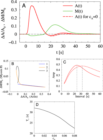
Figure 6. Numerical simulations of equations (2), (3). (A) Dynamics of A(t) (actin) and M(t) (myosin II) for the regime of damped oscillations after a single stimulation at t = 0. Dynamics of actin in the absence of coupling with myosin II, cA = 0, dashed line (myosin II-null cells) shows slower relaxation. (B) Trajectory in the A–M (actin—myosin II) plane with three phases of the dynamics. (C) Resonance curves for the amplitude of A(t) (actin) response under periodic stimulation. The resonance period in the absence of coupling with myosin II dynamics, cA = 0 (dashed line), is longer than for  . (D) Resonance period of actin response as a function of the coupling strength cA with myosin II dynamics.
Download figure:
Standard image High-resolution image5. Discussion
The main driving forces for amoeboid cell movement are generated by the actomyosin cytoskeleton, in particular, the actin network. To study the coupling dynamics between myosin II and F-actin, we applied a receptor stimulus of precisely controlled timing and then investigated the response dynamics of fluorescently labeled myosin II and F-actin in detail. Our work did not aim at revealing new mechanistic details of the biochemical signaling pathways that regulate actomyosin dynamics. Instead, we analyzed the response kinetics in a dynamical systems framework that yields quantitative insight into how actin, myosin, and area contraction of the cells are correlated. Moreover, we developed a dynamical model that allowed us to explore various mechanistic relations, such as the effect of coupling between myosin and actin dynamics.
Our experiments showed that immediately after stimulation with cAMP, actin filaments grow in the cortical region whereas myosin II is released from the cortex. As myosin II inhibits the formation of pseudopods [11–13, 53, 54], the release of myosin II from the cortex during this stage allows the freshly formed filamentous actin to protrude the membrane more effectively. Most proteins in the chemotactic signaling pathway (such as PH domain proteins and Ras) or the regulatory actin network (such as Aip1, Arp2/3, coronin) are also translocated to the cortex during this time [23, 42, 55, 56] to orchestrate the rapid actin turnover. In addition to previous observations that myosin II responded to the stimulation on a much later time scale (around 30 s after stimulation) [51], our findings show that myosin II is in fact responsive, though less pronounced, already within 10 s after stimulation—it is released from the cortex into the cytosol as a first dynamical response to the stimulation.
We also observed that the later translocation of myosin II to the cortical region is due to the fact that the translocation of myosin II requires filamentous actin. The coupling between the dynamics of myosin II translocation to the cortical region and F-actin is confirmed by the almost linear relation found between the time myosin II reaches maximum accumulation in the cortex and the total time of initial polymerization, followed by depolymerization of cortical actin filaments (see figure C2(C) in appendix C). The delay in the recovery of cortical filamentous actin in myosin II-null cells (figure 5(A)) suggests that the interaction between myosin II and actin filaments not only carries myosin II from the cytosol to the cortex but also enhances the efficiency of actin accumulation in the cortical region. The interaction of myosin II and actin filaments in the cortex leads to cell contraction as the main difference between the morphology of wild-type and myosin II-null cells is also found at the beginning of phase 3, where myosin II and filamentous actin translocate to the cortex together (figure 3).
It is known that an effective cell movement requires three stages: (1) extending cell protrusions towards a preferred direction, (2) attaching the leading edge to the surface as well as detaching the trailing edge from the surface, (3) contracting the uropod to pull the entire body forward [57]. Cells can move effectively under a shallow chemoattractant gradient with the help of directional protrusions and contraction. Under the uniform stimulation used in this study, one can simply assess protrusion and contraction by looking at the area changes as forces produced by actin and myosin II are ubiquitous. We observed that after stimulation, the cell area close to the adherent surface first increases then decreases, and finally relaxes back to the state before stimulation. The first area-increasing stage, due to the growth of cortical actin filaments, protrudes the membrane ubiquitously, resulting in a roundish cell shape. This almost isotropic protrusion also leads to a temporally slowing down and even cessation of random motion, a response usually referred to as cringing [5, 58], which also happens to cells in a steep chemoattractant gradient [59, 60]. The shape change alters the amount of scattered light [61] and is usually used to indicate the propagation of cAMP waves in studying the collective behavior of D. discoideum[62, 63]. It has been reported that myosin II bundles with actin filaments at the cell periphery and thereby supports cell shape and maintains integrity [8, 11]. In the absence of myosin II, actin filaments can only provoke local forces instead of spreading out the force along the membrane lined with myosin II. This could account for the slower area expansion in myosin II-null cells (figure 5(B)). The observation that myosin II-null cells still show the first area-growing phase (figure 5) and cringe response [12, 64] further supports that the first phase of area change is driven by the growth of actin filaments and is only indirectly related to myosin II. The phase trajectories clearly point out that the area-decreasing phase is actually composed of two different mechanism (figures 4(A), (C)): the disassembly of F-actin reduces the support to the expanded membrane, resulting in the first part of area-decrease (phase 2 in figures 4(A), (C)). Then myosin II and F-actin form a complex which contracts and leads to the second part of area-decrease (first part of phase 3 in figures 4(A), (C)).
Our model successfully captures the F-actin dynamics in the absence and in the presence of external stimulation. The simulations reproduce the F-actin dynamics with and without myosin II consistent with our experimental findings (figure 6). Our experiments support that the interaction between F-actin and myosin II not only carries myosin II from the cytosol to the cortex [coupling term in equation (3)] but importantly enhances the efficiency of actin accumulation in the cortical region [coupling term in equation (2)]. In our model the time delay in the coupling, τAM, is only present in the equation for myosin II dynamics [last term in equation (3)]. This time delay reflects the experimental observations that myosin II translocates to the cortex at about τAM later than F-actin starts to grow. The proposed interplay in the model between myosin II dynamics and the F-actin concentration [factor A(t − τAM) in the coupling term in equation (3)] implies an involvement of other regulatory proteins. It has been reported that myosin heavy chain kinase A (MHCK A) is massively translocated to the cortex at the same time as myosin II, i.e. with a delay time τAM ≃ (20−25) s with respect to the F-actin response [50]. MHCK A phosphorylates myosin heavy chain to disassemble the myosin filaments [65, 66]. The significant depletion of MHCK A in the cytosol allows the formation of myosin II bundles there. The attachment of multiple heads of the myosin II bundles to actin filaments allows myosin II to localize with actin filaments persistently and is essential for the translocation of myosin II from the cytosol to the cortex [52, 67]. These factors together contribute to the growth of cortical myosin II concentration. Further experiments with cells that are simultaneously labeled for MHCK A and F-actin should shed more light on the factors determining the delay time τAM in the model. Besides MHCK A, so called contractility kits composed of cortexillin I and the scaffolding protein IQGAP2 that are preassembled in the cytosol of D. discoideumand regulate myosin activity [68], might be relevant for the first, rapid response of the actomyosin machinery to stimulation, as the quick reshuffling within the first 10 s upon stimulation (i.e. between phases 1 and 2), which we have identified.
Our model also demonstrates that the resonance period of actin response becomes more sensitive to the coupling strength when increasing cA (towards wild-type cells), see figure 6(D). This prediction could explain in particular large variability of the total time of polymerization and depolymerization of cortical actin filaments observed in the wild-type cells (see figure C2 in appendix C). For future experiments focused on D. discoideumactin-myosin II coupling upon chemotaxis, in particular to prove whether the resonance period of the actin response follows our predictions, gradual inhibition of the activity of myosin II in a stepwise fashion by the addition of widely used myosin II inhibitor blebbistatin [69, 70] should be possible.
In summary, our findings highlight the role of myosin II in regulating filamentous actin dynamics, as well as cell morphology after cAMP stimulation. The coupled dynamics between actin and myosin II can be seen as a prerequisite for the robust control of cell contraction and movement irrespective of large variations from the environmental stimulus. Future work will concentrate on a more refined, spatially resolved analysis of the interplay between actin, myosin, and shape changes along the cell contour, where fluctuations in the dynamics are expected to play a crucial role.
Acknowledgments
This work was supported by the Max Planck Society and the German Research Foundation (DFG) Grant No. SFB 937 'Collective Behavior of Soft and Biological Matter' project A09.
Appendix A.: Periodic stimulation
To facilitate the observation of phase locking we have used periodic stimuli. When the stimulation interval was short (11 s, figure A1(A)), the responses only explored phase 1 (figure A1(C)). Longer stimulation intervals allowed the responses to explore more of the phase space. When we extended the stimuli interval to 21 s (i.e. approximately the time duration of phase 1 plus phase 2, figure A1(B)), the trajectories formed a closed loop, composed of the straight line in phase 1 and the circular arc in phase 2 (figure A1(D)). The trajectories from consecutive responses are similar (gray lines in figures A1(C) and (D)) and comparable with the trajectory from the averaged response signal after a single pulse stimulation (figure 4(A), the fitting from phases 1 and 2 are plotted here as black lines).
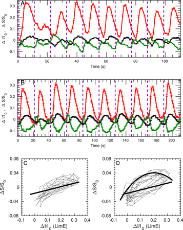
Figure A1. Dynamics of F-actin and myosin II in response to periodic stimuli of cAMP. In (A) and (B), red traces show the signal of F-actin (LimE-mRFP), green traces show the signal of myosin II-GFP and black traces show the signal of area change. Purple dashes show the application time of cAMP stimulation. Error bars are standard error of the mean. (A) Responses to periodic stimulation with an interval of 11 s, N = 13 cells. (B) Responses to periodic stimulation with an interval of 21 s, N = 15 cells. (C) Relation between F-actin and area for the data in (A). Black line is the fit of phase 1 from figure 4(A). (D) Relation between F-actin and area for the data in (B). Black line is the fit of phases 1 and 2 from figure 4(A).
Download figure:
Standard image High-resolution imageMyosin II decreased slightly right after cAMP stimulation (figure 3), suggesting a release of myosin II from the cortex. To further confirm its release, we enhanced the response signal: As myosin II gradually accumulated in the cortex during 15–25 s after cAMP stimulation, another stimulation in this interval would triggering release of more cortical myosin II. We therefore stimulated cells co-expressing LimE-mRFP and myosin II-GFP periodically. While the signal of LimE-mRFP (red traces in figure A1(B)) always increased after cAMP stimulation, myosin II-GFP (green traces in figure A1(B)) always decreased after stimulation. This confirms the release of myosin II fro the cortex after cAMP stimulation.
The results of numerical simulations of equations (2), (3) for the periodic stimulation in the regime of damped oscillations are shown in figure A2 for comparison. The model reproduces the typical shape of the response signals found in the experiments.
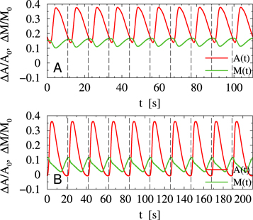
Figure A2. Numerical simulations of equations (2), (3) for periodic stimulation with an interval T = 11 s (A) and T = 21 s (B). Vertical dashed lines show the time of stimulation.
Download figure:
Standard image High-resolution imageAppendix B.: Self-sustained oscillations of F-actin and myosin II
To investigate the role of myosin II on autonomous oscillations of filamentous actin, we first inspected the dynamics of F-actin and myosin II in cells with LimE-mRFP and myosin II-GFP in the absence of external stimulation. The oscillations of LimE and myosin II were found independent of each other: (i) cells showing oscillations only in LimE, but not in myosin II; (ii) only in myosin II, but not in LimE; (iii) in both LimE and myosin II. Typical dynamics of the LimE-mRFP and myosin II-GFP signals for these three cases is shown in figure B1 in the left column with the results of numerical simulations of equations (2), (3) on the right. In figure B1(A) self-sustained oscillations of LimE were not accompanied by myosin II oscillations. In figure B1(B) only spontaneous oscillations of myosin II-GFP signal were observed. Finally, figure B1(C) gives an example of simultaneous self-sustained oscillations of LimE-mRFP and myosin II-GFP.
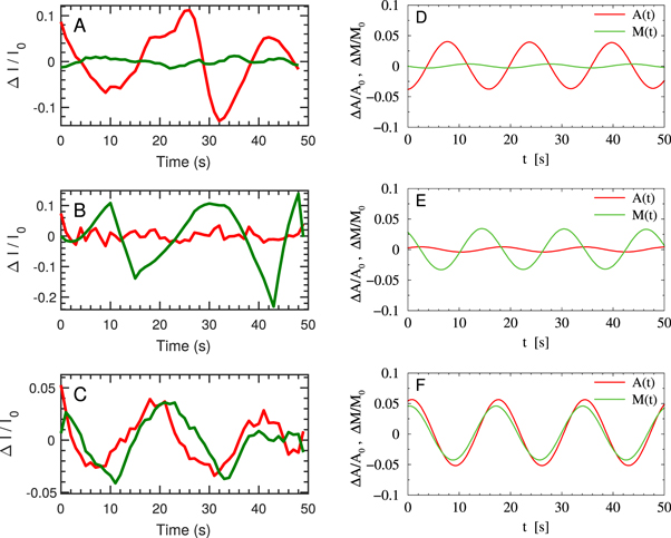
Figure B1. The dynamics of F-actin and myosin II are independent of each other in the regime of self-sustained oscillations. Red traces are LimE-mRFP (F-actin label) signals and green traces are myosin II-GFP signals. (A) An exemplary cell showing F-actin oscillations without myosin II oscillations. (B) An exemplary cell showing myosin II oscillations without F-actin oscillations. (C) An exemplary cell showing both F-actin and myosin II oscillations. (D-F) Numerical simulations of equations (2), (3).
Download figure:
Standard image High-resolution imageTo reproduce these scenarios in numerical simulations we had to change the model parameters  and
and  in such a way that the corresponding conditions for the Hopf bifurcation are satisfied (see section 4 for details). The results shown in figure B1(D) corresponds to
  ,
,  , in figure B1(E)
  ,
,  , and in figure B1(F)
  ,
,  .
.
Appendix C.: Coupled dynamics of F-actin and myosin II
We examined the effect of cortical myosin II on actin dynamics by analyzing the responses of individual cells to a single 1 s stimulus with the concentration of uncaged cAMP ranging from 100 nM to 100 μM. The difference between maximum and minimum of the LimE signal (A in figure C1) reflects the amount of polymerized/depolymerized F-actin, as well as, dissects the actin response time in phases 1 and 2 (Tp and Td in figure C1). In figure C2 the relation between response amplitude of LimE signal and polymerization and depolymerization time is shown together with the relation between the time to reach a maximum of myosin II response, TM, at the beginning of phase 3 (see figure 3) and the total time Tp + Td of LimE response. Each point shows the response of one cell co-expressing LimE-mRFP and myosin II-GFP after a single stimulation. The LimE signal varies in amplitude and time scales within every cell even in response to the same stimulation strength (figures C2(A), (B)). The polymerization time Tp from different wild-type cells stayed constant over the entire range of response amplitude A, whereas the depolymerization time Td increased. The relation between polymerization/depolymerization time and the response amplitude of F-actin signal obtained for myosin II-null cells were the same as for wild-type cells (figures C2(A), (B)). This suggests a similar underlying mechanism controlling the dynamics of filamentous actin in the absence of myosin II. Thus the dynamics of cortical myosin II has no effect on the actin dynamics in the phases 1 and 2 after stimulation.

Figure C1. Schematic presentation of F-actin response to a single stimulation at t = 0. The time interval to reach a maximum after stimulation is the polymerization time, Tp. The time interval from maximum signal to minimum is the depolymerization time, Td. The signal amplitude between maximum and minimum is A.
Download figure:
Standard image High-resolution image
Figure C2. (A) Polymerization time Tp as a function of the amplitude of the LimE (F-actin label) response signal. (B) Depolymerization time Td as a function of the amplitude of the LimE response signal. (C) Coupled dynamics between myosin II and F-actin. Time to reach a maximum of myosin II response after stimulation, TM, as a function of Tp + Td of LimE signal. Black crosses—wild-type cells, blue crosses—myosin II-null cells. (D)–(F) Results of numerical simulations of equations (2), (3).
Download figure:
Standard image High-resolution image
However, the time for myosin II response to reach maximum in the cortex (TM of myosin II-GFP signal) is closely related to the total time of polymerization and depolymerization of cortical actin filaments (Tp + Td of LimE signal) (figure C2(C)). This suggests that a robust coordination emerges from the interaction between actin filaments and myosin II bundles, which further allows precise control of cell contraction in phase 3.
Numerical simulations of equations (2), (3) show a good agreement with the experimental results (figures C2(D)–(F)). Note that in the simulations only the stimulation amplitude was varied and cell-to-cell variability was not taken into account.