


Abstract
The investigation of separable states in quantum theory has been driven by the notion that they are highly classical, in that they do not demonstrate nonlocality, and are in some contexts unable to support non-classical computation. The converse question, the extent to which entangled states do or do not support non-classical information processing, is less well understood. Motivated by this question we extend the notion of quantum separability into the entangled quantum states, by constructing separable decompositions that describe them with the 'smallest' possible sets of non-physical local operators. We consider a few ways to define the word 'smallest' and present techniques for obtaining them. The methods involve calculating certain forms of cross norm. The results generalise significantly the results obtained in our previous work on this topic (2015 New J. Phys. 17 093047), and can be be used to construct classical simulation methods and local hidden variable models for subsets of local measurements on entangled quantum states.
Export citation and abstract BibTeX RIS

Original content from this work may be used under the terms of the Creative Commons Attribution 3.0 licence. Any further distribution of this work must maintain attribution to the author(s) and the title of the work, journal citation and DOI.
1. Background and overview
A central goal of quantum theory is to determine when quantum systems can or cannot be described by a 'classical' model. The term 'classical' can be defined in many ways, but in the context of multipartite quantum systems two of the most common definitions are a 'non-locality' definition, in which a system is described as being classical if it has a local hidden variable model [1, 2], or a 'computational complexity' definition, in which a system is described as being classical if it can be simulated efficiently using a classical computer [3–5].
The notion of quantum entanglement plays an important role in studies of these problems. In the context of non-locality, for example, it is easy to show that if a state  of particles
  is not entangled, i.e. it has a separable decomposition

where the pk form a probability distribution and the  are local density operators, then it has a local hidden variable model [6]. The converse is not true, in that there are entangled, non-separable, quantum states for which there are local hidden variable models for all local measurements [1, 6, 7]. Similarly, in the context of computational complexity, it is known that if a device consists of non-entangling quantum gates acting on product input states [8], then the device can be efficiently simulated classically. Hence in the context of gate-model quantum computation, entanglement is also necessary for non-classical computation, although in more general models of quantum computation this might not be true (e.g. even sampling thermal states of classical many-body systems cannot always be performed efficiently [9]).
The intuition behind such classical models and simulation algorithms is that for non-entangled systems the correlations are mediated entirely by the classical probabilistic weights pk, followed by extra 'local' sampling of the measurement of the local density matrices. When the classical weights can be efficiently sampled classically, as has been shown to be the case for gate model computers with non-entangling gates [8], then the extra step of sampling the local outcomes from the  is not computationally expensive. Similarly, for local hidden variable models the index k serves as the classical hidden variable, and the local
  provide the local response functions.
Motivated by these observations, in this work we will consider extending the notion of a separable decomposition to entangled quantum states in order to find new ways of constructing classical models. The way that we will extend the notion of separability is by relaxing the requirement that the local  be quantum states (e.g. by relaxing the requirement that they be positive). This will permit us to find 'generalised separable' decompositions for entangled quantum states. Without any further considerations this would be a trivial task, as any multipartite operator can be expanded as a probabilistic sum of non-positive operators. However, we will be interested in looking for decompositions in which the local operators are 'as positive as possible', with the aim of eventually using them for classical models. This naturally leads to the question, what criteria should we use to assess 'as positive as possible'? An approach that we took in our previous investigation of this problem [10] was to look for separable decompositions involving small sets of local operators, primarily for describing maximally entangled states. In this work we will extend those results significantly, in some cases to all bipartite quantum states. The results we present will show that separable decompositions of non-entangled quantum states are part of a more general family of separable decompositions, which at the other extreme of entanglement includes discrete Wigner function local hidden variable models for maximally entangled states. As with [10], our results are strongly connected to the notion of cross-norms that has been applied to entanglement theory [11, 12].
Our results may be summarised as follows: (i) for any bipartite entangled states we compute all cross-norm achieving decompositions for certain families of cross norm, (ii) on the basis of these decompositions we construct local state spaces for which a given bipartite entangled state is separable, such that the state spaces cannot be made smaller while still supporting a separable decomposition, (iii) for some families of bipartite state we find separable decompositions involving state spaces that are the duals of the largest possible sets of local measurements. Our hope is that in future work these methods will provide useful alternative descriptions of bipartite quantum states for use in classical models, such as generalisations of discrete Wigner functions local hidden variable models, or as alternative variables in classical simulation algorithms.
Structure—This paper is structured as follows. In the next section we discuss the relationship of our work to other literature. In sections 3 and 4 we describe at a broad level the idea of generalised separability, and present some separable decompositions for Bell diagonal states that illustrate and motivate the problems that we will address in this work. In section 5 we describe in detail the four problems (Problems 1, 2, 2*, 3) that we consider. In section 6 we describe some norms and notation that we use. In section 7 we present a brief list of our main results, which constitute three Theorems. Theorem 1 characterises all solutions to Problem 1 for all bipartite states for all norms that we consider. Theorem 2 solves Problem 2 for all bipartite states. Theorem 3 presents solutions to problems 2* and 3 for certain families of bipartite state (including the pure states in a region around the maximally entangled state). The proofs are presented in sections 8–10. They may be skipped by those not interested in the proofs. The appendix contains a brief discussion of some notions of generalised positivity.
2. Relationship to other work
To set the scene it is useful to compare our results to related literature in the foundations of physics, entanglement theory, and quantum information. In an attempt to understand why quantum theory permits highly non-classical correlations, various authors have investigated the kinds of correlations that can occur in hypothetical theories more general than quantum theory. In the study of generalised probabilistic theories [13, 14] for example, various reasonable axioms are postulated for physical theories (such as no instant signalling), without necessarily demanding that the theory has an underlying Hilbert space or operator space structure. In such theories correlations can arise that are stronger than quantum [14, 15], and the question of why such correlations do not seem to occur in nature has attracted much attention. One way of constructing such non-quantum theories is to start from a quantum setting in which local parties can only perform quantum measurements in certain restricted directions, but then to allow the joint states in the theory to be represented by non-positive and hence non-quantum operators (e.g. allowing them to have negative eigenvalues [16]). As long as the measurements are restricted so that the Born rule gives only positive numbers, then the non-positivity of the states will not show up in any calculations, and the theory will yield valid probabilities. The correlations obtained in this way can be stronger than in quantum theory [16].
In a similar vein, in this work we will consider 'state spaces' that do not consist of positive quantum states. However, in contrast to these works, in this article we will only consider joint states that are physical quantum states (even though our results apply to some non-quantum joint states too), instead it will be the local state spaces that are not quantum (e.g. containing operators with negative eigenvalues). Our motivation is hence not whether the correlations are stronger or weaker than quantum correlations, but is more in the spirit of the use of Wigner functions [17] in the discrete setting [18], in which non-positive operators can be used to provide classical local hidden variable models for mutually unbiased basis measurements [19]. A related motivation comes from the work of [20], which studied the nature of entanglement when the local observables are restricted to certain algebras. Settings with restricted local measurements are physically important because in most applications the measurements available will be restricted due to technological constraints, selection rules, imperfections, or by design in order to enable quantum error correction.
We will however not start with a specific set of measurements or dynamical processes in mind. We will instead start with a given bipartite entangled and usually non-local state, and ask how we may represent the state so that the largest set of measurements or processes may be considered classical. In formulating this problem we will draw upon our previous work on this topic [10], which drew connections with the use of cross norms [11, 12, 21] to study entanglement. This will supply us with the main technical tools that we need. Our previous work [10] primarily focussed on maximally entangled states and some bipartite pure ones. The results we derive here are much more general. Some of the problems we consider have natural mathematical parallels in the study of decompositions in theory of frames [22, 23].
Our original motivation for this work was to understand the extend to which the notion of separability can be applied to entangled states, with the aim of developing new variables that could be useful in the classical description of quantum systems, e.g. in the description of valence bonds in PEPS states [24–26]. However the separable decompositions we present can also be used to construct local hidden variable models for restricted sets of measurements. However, in this sense our models are weaker than other models in the literature—it has long been known that there are entangled quantum states for which there are hidden variable models for all measurements [6, 7], and more recently systematic algorithms have been developed for constructing local hidden variable models where they exist [27]. These methods typically make no (or few) restrictions on the measurements. However, the separable decompositions that we present do have some appealing properties—they are simple analytic models that are a continuation of separable decompositions into the entangled states, they apply broadly, and they do not depart from the linear structure of quantum theory. The linearity in particular may make it easier to use these models as building blocks to describe more complex systems.
3. Motivating example: discrete Wigner representation of Bell states
It has been known for many years [2] that Bell pairs of two qubits, such as the state

have local hidden variable models for local measurements of the Pauli operators. In this section we will review this result in the light of a generalised notion of separability. Given the Pauli measurements in the  and z directions, one can define a 'dual' set operators as those operators of unit trace which return positive probabilities for these measurements under the Born rule, i.e. the set of operators

where the 'Pauli' denotes the set of six projectors onto the Pauli measurement eigenstates, and the * is used to denote the dual set. In some situations it is convenient to remove the restriction that the operators be normalised to unit trace, in which case the set becomes a convex (blunt) cone (i.e. a set that is closed under linear combinations involving positive coefficients—sometimes non-negative coefficients are allowed, in which case the cone is said to be 'pointed' rather than 'blunt'). However for the purposes of the present discussion we will include the requirement of normalisation. This means that for our purposes the set of dual operators is a convex set, but not a cone.
The normalised dual set Pauli* of the Pauli measurements can be visualised as a cube of Bloch vectors enclosing the Bloch sphere, and so for brevity we will refer to the set Pauli* as the 'cube'. Although the cube contains non-positive and hence non-physical operators, if we are considering only Pauli measurements, then these operators give valid probability distributions under the Born rule, and hence can be used to construct local hidden variable models, just as the local quantum states do for separable states of the form of equation (1). Indeed this can be done for the Bell state of equation (2), as its density matrix can be written in a 'cube-separable' form [10, 18]

where the Wi and their transpositions WiT are examples of so-called phase-point operators [18] that arise in the study of discrete analogues of Wigner functions. The Wi and WiT are defined by the following equations
where  are the Pauli
  and z operators. Although the Wi and WiT are not quantum states as they are not positive, they are unit trace operators and they correspond to certain corners of the cube. Hence we may say that the decomposition (3) furnishes a cube-separable decomposition for
  , and consequently it supplies a local hidden variable model for Pauli measurements. In passing we note that any two qubit quantum state that has a local hidden variable model for Pauli measurements must have a cube-separable decomposition [28], and these constructions can be generalised to maximally entangled states of any dimension of particles, under mutually unbiased basis measurements [28, 10, 18].
However, as we shall now see, there is an alternative way of viewing equation (3) that leads to a local hidden variable model for much more than the Pauli measurements. The reason for this is that the convex hull of the operators  in fact corresponds to a 'tetrahedron' of Bloch vectors with vertices given by four of the corners of the cube (similarly the convex hull of the
  gives a tetrahedron aligned in a different direction for the second qubit). As these tetrahedra are smaller than the cube, they are actually the duals of a larger set of measurement operators containing more than just the Pauli measurements. For instance, in addition to the Pauli measurements on the first qubit we may allow POVMs of the form:

where c satisfies  and where
  is the state with Bloch vector
  (sometimes referred to as a type of 'magic' state as it brings the power of quantum computation to some architectures that otherwise can be efficiently simulated classically [29]). Similarly we may allow POVMs that are the transpositions of these for the second qubit. As the 'tetrahedron-separability' of
  furnishes a local hidden variable model for any set of measurements for which the tetrahedron is the dual, these extra measurements can be included in the local hidden variable model in addition to the Pauli measurements.
These observations motivate the primary goal of this work: loosely speaking we aim to systematically find 'good' separable decompositions for bipartite entangled quantum states. Our hope is that they will lead to not only analytic local hidden variable models, but also classically efficient simulation methods for some types complex quantum systems (see e.g. [24] for an example approach). While we will consider a number of different definitions of the word 'good', one of the main guiding principles will be that the decompositions should involve local state spaces that are as 'small' as possible. In order to illustrate the kinds of results that we will obtain, in the next section we will present a family of separable decompositions that generalise the above tetrahedral-separable representation of pure Bell states to all Bell diagonal mixed states. In doing so we will be able to discuss the senses in which our decompositions are optimal.
4. Example decomposition: Bell diagonal qubit states
Bell diagonal mixed states are the two qubit states that are diagonal in the Bell basis:

In [30] it is shown that quantum states that are diagonal in this basis may be given the following representation:

where  are three real parameters. The representation gives a valid quantum state when the vector
  of parameters is drawn from the convex hull of
  . Within this convex hull the vectors with
  correspond to quantum separable states, while the pure maximally entangled Bell states have
  (please note that although the convex hull of the
  is a tetrahedron, it is conceptually distinct from the tetrahedra described elsewhere in this work, which are defined with reference to only one state particle, not two). For convenience we rewrite the representation (6) as follows

where we have absorbed any negative signs into the  of the second qubit, calling the resulting operator
  . Consider a given Bell diagonal state
  . The techniques we describe later in this paper can be used to write down the following 'separable' decomposition for the state:

where
and the Bk are defined through the same expressions, but replacing σ with  . We define the 'local state space' for particle A as the convex hull of the Ak and for particle B as the convex hull of the Bk, and we denote these state spaces as VA and VB respectively. We describe the decomposition (8) as a 'separable decomposition for
  w.r.t. VA and VB'. The state spaces are all 'tetrahedral' (i.e. simplices) in shape, and the operators Ak and Bk interpolate between the discrete Wigner representation for pure Bell states when
  at one extreme, and quantum-separable decomposition when
  at the other, corresponding to the threshold at which the Bell diagonal states become quantum-separable. In this sense we see that the ordinary notion of quantum separability seems to have quite natural analogous extensions for all Bell diagonal quantum states, matching the discrete Wigner representation (3) in the extreme case of pure Bell states.
As we will prove later, provided that an odd number of the ti are non-zero (which is generically the case), the decompositions described by equation (6) have a number of notable properties which we think of as being 'good':
- 1.The operators appearing in the decompositions (8) have the smallest norm possible, in the sense that it is not possible to provide a separable representation of any given
 involving operators of lower average 2-norm.
 - 2.No convex strict subsets of VA and VB admit a separable decomposition for any given, i.e. the local state spaces cannot be made any smaller while admitting a separable decomposition for .
- 3.Consider the largest sets MA and MB of measurement operators for which VA and VB are the unit trace dual sets respectively. For a given is not possible to add any further measurement operators to the sets MA and MB such that the state remains separable w.r.t. to the new dual spaces. Equivalently if one constructs state spaces from VA and VB by taking the convex hull of the unions with the local quantum states (see figure 1), then no smaller convex state spaces can be found that contains the quantum states while admitting a separable decomposition for . The proof of this and the previous property will be presented in footnote6
, as it requires a slight modification of the arguments presented in the main text.


These three properties illustrate the three main notions of 'goodness' that we will use to identify separable decompositions for bipartite entangled quantum states, and the goal of this work will be to find decompositions for entangled quantum states that share these properties. All three notions were considered in our previous work [10], where we derived separable decompositions with these properties for certain families of bipartite pure state. In this work we extend these results to much larger classes of state: we obtain all separable decompositions achieving the first property for all bipartite states, we obtain separable decompositions achieving the second property for all bipartite states, and we obtain separable decompositions achieving the third property for some bipartite states.
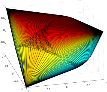
Figure 1. The image illustrates a convex hull of a tetrahedron and the sphere of quantum Bloch vectors. The tetrahedron is the convex hull of the phase point operators in the discrete Wigner representation. This local state space is a solution to Problem 2* for Bell states.
Download figure:
Standard image High-resolution image5. Definitions and Problems considered
Consider a convex set of local operators  acting on system A, and convex set of local operators
  acting on system B. We say that a bipartite state
  is
is  -separable, or that
  is separable w.r.t.
  , or that
  separate
  , if there is a decomposition of the form:

where the pk form a probability distribution, and the Ak and Bk are operators drawn from  and
and  respectively. We refer to
  and
and  as 'local state spaces'. In the literature a bipartite quantum state is usually said to be separable if it has a separable decomposition w.r.t. local quantum state spaces (i.e. the local unit trace positive operators). However, to distinguish this notion from more general
  -separability we will call such states quantum-separable rather than just separable.
If we are to attempt to use the decomposition to provide a local hidden variable model for an entangled quantum state, or to provide a route to a classical simulation algorithm, then we would like to find decompositions involving local state spaces that are 'positive enough' for whatever our intended purpose is. There are many inequivalent ways of defining the phrase 'positive enough', depending upon the measurements or dynamics that one is considering. In the earlier examples of local hidden variable models, we saw that 'positive enough' meant being contained within the dual set of the measurements being considered. However, there are many inequivalent sets of measurements that one may consider, and moreover, if instead of local hidden variable models one seeks variables to use in classical simulation algorithms, then other notions of positivity can apply (see e.g. [24], and appendix). In spite of the wide variety of possible generalised definitions of positivity, many of them have the property that if a set of operators is positive, then so is any subset of it. This means that if we have two candidate separable decompositions for a given quantum states, such that the local state spaces for one decomposition are contained strictly within the local state spaces of the other, then the former decomposition will be preferred as the local state spaces can only be 'more' positive. The comparison of cube and tetrahedral separability for the pure Bell state was an example of this: the smaller tetrahedral state space was preferred as it provided a more powerful local hidden variable model.
Our main aim in this work will hence be to find 'small' separable decompositions for entangled quantum states. There are four variants of this problem that we will consider, depending upon different definitions of the word 'small', although two of them (Problem 2* and Problem 3 below) are equivalent and are defined separately for later convenience. All four problems were considered in our previous work [10], where solutions were presented primarily for maximally entangled states. In this work we will generalise those results significantly. The problems are defined as follows.
- Problem 1: for a given bipartite quantum state consider all pairs of local convex state spaces for which is separable, and work out the minimum (in all cases considered in this paper the minimum exists) value of , where we define the size of a state space relative to some choice of norm as , which can be of a different form for each subsystem A and B.


In [10] this was shown to be equivalent to computing a form of cross-norm [11, 12] built from  (readers that are not familiar with cross norms may see equation (17) for a definition of the versions that we consider here). Depending upon the choice of norm, this problem may not have strong physical meaning by itself. However, we use it as a mathematical tool to solve the other variants of the problem that we consider. As discussed above, the generalised positivity of a set of operators usually implies generalised positivity of any of its subsets, so it is in our advantage to look for separable decompositions involving local state spaces that cannot be made smaller. This motivates the second of our problems.
- Problem 2: for a given quantum state , consider all pairs of convex state spaces for which is separable, and identify pairs such that no strict convex subsets or exist for which is -separable.


Problems 1 and 2 contain a couple of drawbacks that we remedy by defining the following two problems, Problem 2* and 3. While Problem 2* and Problem 3 were both considered in [10], only Problem 3 was explicitly defined there. However they are mathematically equivalent.
- Problem 2*: the same as Problem 2, but with the additional constraint that we identify smallest state spaces under the restriction that they must contain the local quantum states and they only contain operators with unit trace.
- Problem 3: the same as Problem 2, but with the additional constraint that the state spaces must be convex cones of positive trace operators that contain the quantum states (in this case the weights appearing in the separable decomposition need only be positive—whether they form a normalised probability distribution is irrelevant as we are now dealing with cones). The motivation for this problem is explained in [10], but for convenience we recap the idea in footnote7
. Problem 2* and Problem 3 are mathematically equivalent because the conic hulls8
of solutions to Problem 2* automatically give solutions to Problem 3, and a unit trace slice through a solution to Problem 3 gives a solution to Problem 2*.

Problem 3 is only included here as it is expressed in terms of the language of conic sets, which is sometimes a more natural framework in which to consider generalisations of quantum theory [20]. However the problem we will consider directly is Problem 2*. The reasons for defining these modified problems is to address two drawbacks with Problems 1 and 2. The first drawback is that they do not consider the fact that local quantum states may be freely used in the separable decompositions because they are positive under any notion that we will consider. This means that if one set of separating local state spaces differs from another set simply by containing (convex combinations) with additional local quantum states, it should be considered equally 'good', even though it involves larger state spaces. This is why we have added the requirement that the state spaces contain the local quantum states. Moreover as discussed in [10], including the requirement of the local quantum states means that if we have a solution to Problem 2* it is not possible to find smaller separating local state spaces for which the dual is a larger set of local measurements. The second drawback with Problems 1 and 2 is that some solutions lead to local operators of zero trace, for instance the decomposition
of the Bell state (2) is a solution to both Problem 1 (for an appropriate choice of norm) and Problem 2. However the  cannot be generalised positive for a complete POVM other than the trivial identity measurement, as they are traceless. Including the requirement of unit trace in Problem 2* means that, provided that the local operators are Hermitian and bounded (which can be easily enforced for most of the constructions that we present), there will be some non-trivial POVMs (e.g. ones with measurement operators almost proportional to the identity) for which the state spaces is dual.
In order to solve these problems we will need to exploit connections to certain families of cross-norm, which we define in the next section, alongside the notation that we use.
6. Cross-norms and notation
In this work we will characterise the local operators and the entangled state using norms that are given by the 2-norm of the output of fixed invertible linear transformations. We denote them in the following way:

where Λ is an invertible linear transformation (which will always be displayed in upper case, although the font may vary), and  refers to the 2-norm of
  (the 2-norm of an operator Y is defined as
  ).
).
As described in the description of Problem 1, we can use norms such as these to define the size of sets  of operators via the definition
There are two reasons why norms such as (14) are useful to us: firstly the triangle inequality is strict for them, i.e.

unless X = cY for some positive number c9
, and secondly we can often calculate the so-called cross norms [11, 12, 21] resulting from them explicitly, as well as all cross norm achieving decompositions. Given two invertible linear transformations  we define the
  cross-norm as:

The arguments presented in [10] show that minimising  such that
  is
is  -separable is equivalent to calculating a cross norm of
  . In particular the following identity holds

where the infimum is taken over all pairs of sets  such that
  is
is  -separable.
We will utilise the fact (in analogy to the Schmidt decomposition or Singular value decomposition for pure quantum states) that a bipartite density matrix may be given an operator Schmidt decomposition, i.e. it can be written as:

where the Xi and Yi are orthonormal operators bases (i.e.  ), the operator-Schmidt coefficients si satisfy
  , and the operator-Schmidt rank is given by D, which satisfies
  , where
  and
and  are the dimensions of particle A and particle B respectively. In the rest of this work will usually assume that
  , but the arguments can easily be extended to all permissible values of D and all finite dimensions.
We will also use the basis occurring in the operator Schmidt decomposition to represent linear operators on each subsystem. Consider an operator A on the first particle and an operator B on the second particle. We may expand

where the  form a vector of expansion coefficients, which we will denote by bold font (column) vectors
  and
and  . The complex conjugate is included on the bi for later convenience. In this representation the norms are given by:

where  denotes the usual complex Euclidean norm of vector
  .
.
7. Summary of results
In this section we list the main results of the paper. Proofs are deferred to later sections.
Theorem 1. (All Solutions to Problem 1 for some cross norms) Consider a bipartite quantum state  with operator-Schmidt decomposition
  with
with  . Define
  and make arbitrary choices of the following: positive constants
  , and a D × N isometry U (i.e.
  ). Then

with

gives a  achieving decomposition, which is given by
  . Moreover, all
  achieving decompositions can be written in this form. For the more general cross norms
  all achieving decompositions can be computed by applying
  to the achieving decompositions of
  . Given any of these cross norm achieving decompositions, all separable decompositions solving Problem 1 may be computed through the 'normalising' procedure presented in equation (41).
Theorem 2. (Solutions to Problem 2) Consider a bipartite quantum state  with operator-Schmidt decomposition
  with
with  . Then any separable decomposition of the form

with the Ak linearly independent and the Bk linearly independent is a solution to Problem 2, in the sense that the sets:
cannot be made smaller (w.r.t. set inclusion) while continuing to be both convex and to admit a separable decomposition for  .
.
More explicitly, if we define  and a D × D square invertible matrix
  then
then

gives a separable decomposition for  that solves Problem 2. By choosing the matrix elements of
  to be
to be  and
and  we find that the operator-Schmidt decomposition itself is a solution to Problem 2.
We note that there are close parallels between theorems 1 and 2 and theorems on ensemble decompositions of density matrices (see [32] and theorem 2.6 in [5]). The reasons for these connections will be discussed in the proofs.
Theorem 3. (Solutions to Problem 2* and Problem 3 for some states.) For all bipartite states it is possible to choose the  appearing in equation (25) so that the operators
  are of unit trace. For bipartite pure states in a region around maximally entangled states, the convex hulls of the operators Ak and Bk in equation (25) provide solutions to Problem 2* provided that the pk are picked to be uniform (i.e. all equal to each other), and
  is an orthogonal matrix taking the real vector with coefficients
  (which is a unit vector for bipartite pure states) to the unit vector with components
  .
.
8. Proof of theorem 1: characterisation of solutions to Problem 1 for some cross norms
Before we present the proof of theorem 1, we present a derivation of a result proven in [11, 12]. This will help us to establish notation and adapt the result later in the paper.
Lemma 4. Let the operator Schmidt decomposition for  be
be

with  and
and  . Then the
  cross-norm (which is usually called the projective cross 2-norm) of
  is the sum of the operator Schmidt coefficients

with  .
.
Proof. We present the proof under the assumption that  . It is straightforward to modify the argument for the general case. Consider any finite decomposition of
  into product operators

For any such decomposition we will show that  is lower bounded by
  . We may expand the operators En,Fn in terms of the
  as follows


Then

where  and
and  are vectors of the expansion coefficients. Now,
  also has an operator Schmidt decomposition

In order for the two decompositions (28) and (32) to be equal, the following condition must hold

Summing both sides over i = j we obtain

where the right inequality follows from the Cauchy–Schwarz inequality. The sum of the operator Schmidt coefficients  therefore gives us a lower bound for the usual cross 2-norm
  , but since this lower bound is in fact achieved with the decomposition (32), the inequality (34) is tight. □
This result was proven in [11, 12]. However we will now extend this result by finding all decompositions achieving the cross norm, by drawing upon parallels to the task of finding decompositions of positive operators [32]. We will then apply the result to obtain all cross norm achieving decompositions for the other cross-norms that we consider. These results will later be used to provide solutions to Problems 2 and Problems 2*/3.
Our task is to work out all finite decompositions (28) such that

From the proof of lemma 4, we see that this is achieved iff the Cauchy–Schwarz inequality in equation (34) is saturated, i.e.

for all operators in the decomposition. This is in turn the case iff the vectors representing each operator for each n are proportional:

for some positive numbers cn that may depend upon n. Substituting this into equation (33), and defining the matrix

gives

Hence a decomposition achieves the cross norm  iff it solves equation (38). This corresponds to finding a positive decomposition of the matrix on the left-hand side. To do this we may draw upon previous results on decompositions of positive matrices [5, 32] to find all possible solutions. Defining the D × N matrix Z with components

then equation (38) may be rewritten

Solving for Z gives:

where U a D × N isometry satisfying  . Hence a decomposition (28) achieves the cross norm iff for some positive coefficients cn and a D × N isometry U we may write:
As shown in [10] these solutions automatically lead to solutions to Problem 1. For the reader's convenience we recap the reasons here. Any cross-norm achieving decomposition can be 'normalised' to a separable decomposition in which each term itself has a product norm equal to the cross norm:

In this equation the product terms each have norm  individually, and the pn form a probability distribution defined by

Any solution to Problem 1 for which the norm used is the usual 2-norm can be obtained in this way.
We may use these solutions to construct all solutions to Problem 1 for the other cross norms that we consider. Suppose that we would like to compute the decompositions that achieve the cross norm:

If we define an operator (not necessarily a density matrix):

then it is clear that

The reason for this is as follows. Suppose we have cross norm achieving decompositions

that achieves  . Then because
it must be the case that
However the reverse inequality also holds, because any optimal decomposition achieving  :
:
gives
and so:

Hence all  achieving decompositions can be constructed by first constructing all decompositions achieving
  using the methods described above, and then applying the inverse transformations
  and
and  . Moreover, using the fact that cross norm achieving decompositions are equivalent to separable decompositions solving Problem 1, all solutions to Problem 1 for these norms may be achieved in this way.
9. Proof of theorem 2
We will now show that some of the decompositions of theorem 1 also yield solutions to Problem 2. To do this we first demonstrate two lemmas that will be needed to prove the theorem.
Lemma 5. Consider an operator  (which need not be a density matrix) of operator Schmidt rank D that has an operator Schmidt decomposition of the form

with  forming a probability distribution, and
  . The decomposition is a solution to Problem 2, in that the convex hulls
  and
and  contain no strict subsets that are both convex and for which
  is separable.
Proof. From theorem 1 we observe that  , and that decomposition

achieves it. The sets of operators  and
and  consist of operators of unit 2-norm, and contain the extreme points of
  and
and  respectively. By the strictness of the triangle inequality no other operators in
  and
and  have unit 2-norm. Hence any separable decomposition of
  consisting of operators from
  and
and  must only involve the extremal points
  and
and  . All the extremal points must be involved because the operator-Schmidt rank of
  is D. Hence no convex strict subsets of
  and
and  can admit a separable decomposition for
  . □
. □
Lemma 6. Suppose that  is a smallest separable decomposition for
  in the sense of Problem 2. Suppose that an operator
  of operator Schmidt rank D can be written
  where
where  and
and  are left invertible linear transformations. Then

is a decomposition for  that solves Problem 2, in that
  and
and  contain no convex strict subsets for which
  is separable.
Proof. Suppose some strict convex subsets of  and
and  existed for which
  were separable. Then applying the inverse transformations
  and
and  would give strict subsets of
  and
and  for which
  is separable, which by assumption is not possible. □
To complete the proof of theorem 2 we now note that the existence of left invertible transformations is equivalent to the  and
and  both being linearly independent sets. Indeed, if they are linearly independent then there exist (dual basis) sets of operators
  and
and  such that

Hence if we define:

then  , and the left inverse transformations are given by:

Hence by lemma 6 any separable decomposition:

for which the Ak and Bk are linearly independent supplies a solution to Problem 2. Let us now characterise such decompositions. Using the completeness of the operators Xi and Yi (assuming that  , the arguments can be modified straightforwardly for more general cases) we may pick invertible matrices
  defined such that:


Hence from the operator Schmidt decomposition of  we require that:

Hence we have a decomposition of  in terms of linearly independent operators iff

Explicitly this gives:

which is a equivalent to equation (25).
It is worth noting that these decompositions can also achieve  dependent cross norms, in a similar manner to the solutions to Problem 1: the cross norm corresponding to the inverse transformations
  is achieved by the decomposition.
For completeness we explicitly write the corresponding inverse maps:
10. Proof of theorem 3
To obtain solutions to Problem 2* (and hence also Problem 3) is more difficult than solving Problems 1 and 2. The reason is that solving the problem for all bipartite quantum states would also entail solving the quantum-separability problem, which is known to be NP hard [33]. So we expect to obtain analytical solutions only for a subset of the bipartite states. Nevertheless, our approach to obtaining these solutions will consist of two steps. In the first step we shall attempt to identify solutions to Problem 2 that contain only unit trace operators. We will be able to do this for all bipartite quantum states (in fact the argument works for all bipartite unit trace Hermitian operators). In the second step we will consider the convex hulls of the local quantum states with these state spaces, and show that for sufficiently correlated  the local quantum states cannot participate in a separable decomposition as they have a norm that is too small. Hence a separable decomposition can only involve the original operators, and no strict convex subset of the state space admits a separable decomposition while containing the local quantum states.
Let us begin by identifying solutions to Problem 2 involving unit trace operators only. From equation (57) we see that we must find choices for  and pk such that the operators of those equations have unit trace. This is equivalent to requiring
  and pk to satisfy:
Let us denote the column vector with coefficients  by x, the column vector with coefficients
  by y, and the unit vector with coefficients
  by g. These vectors cannot be arbitrary, for instance the fact that
  has unit trace constrains
  . However, all three vectors can be chosen to be real (by restricting attention to operator Schmidt decompositions over the real space of Hermitian operators).
In terms of this notation we see that we are looking for an invertible matrix  and a real unit vector g (not necessarily with positive components) such that:

The left inequality implies that

Furthermore, as long as  is real, then g will automatically be a unit vector because
  . Hence to find unit trace solutions to Problem 2 we only need to identify an invertible matrix
  such that:

There are infinitely many suitable solutions for  . If x = y, then
  can be any real orthogonal matrix. If
  then the vectors
  span a real two dimensional subspace of
  . Let us define a real orthonormal basis of two vectors q and r for this subspace such that
In this basis the x and y can be written as column vectors:
A real positive matrix that transforms x to y is hence:

where w can be freely chosen as long as the determinant (and hence the matrix) is positive. We may hence pick  to be a real square root of this matrix, extending it as we wish on the remaining
  subspace not spanned by
  .
.
We will now show that in the case of sufficiently entangled bipartite pure states, among these unit trace solutions there are ones that solve Problem 2*. For bipartite pure states the operator Schmidt decomposition can be chosen so that the vectors x and y are equal, and in such cases we may set  to be any orthogonal (real unitary) matrix to obtain unit trace solutions to problem 2. With bipartite pure states the operator Schmidt decomposition can be obtained from the normal pure state Schmidt decomposition
  :
:

where the operator Schmidt values si are now replaced by  . In this decomposition x = y. Hence any orthogonal matrix
  gives unit trace solutions to Problem 2 for pure bipartite states.
We now discuss how to pick these unit trace solutions so that they also solve Problem 2*. The strategy is to consider the inverse transformations corresponding to H:
As discussed in the previous section these maps by construction have the property that

so that:
which shows that  . Note that:
Hence, if it were the case that for any local quantum state Ψ (either of particle A or particle B) that
then adding the quantum states to the local unit trace spaces could not provide any new separable decompositions, and the resulting state spaces would be solutions to Problem 2*.
Let us try to now understand when this is the case. Write  or
or  where the coefficients
  and
and  form vectors that we denote by α and β, which must be of less than unit norm in order to describe a quantum state, so that:
If the pk and  are picked so that the pk are all equal to each other, then these equations become:

These upper bounds are less than 1 whenever  . The maximally entangled state has all
  , so a range of pure states around the maximally entangled state satisfies this.
11. Conclusions
We have considered the construction of separable decompositions for entangled quantum states that are obtained by relaxing the requirement that the local operators in the decomposition be positive unit trace quantum states. The motivation for this problem is the construction of LHV models and classically efficient simulations for bipartite entangled quantum states, or the multipartite quantum states that are built from them.
In this context it is of interest to find 'smallest' decompositions, where the sets of local operators cannot be made smaller while continuing to allow a separable description. We consider four variants of this problem. The first (Problem 1) uses norms to quantify how 'small' a set of operators is. The second (Problem 2) uses set inclusion (so that one set is smaller than another if it is contained within it). The third (Problem 2*) and fourth (Problem 3) variants we add restrictions (requiring the sets to be unit trace, contain the quantum states, or be cones) that are important when constructing classical models. For the first problem we present all solutions for bipartite states for some norms For the second problem we present some solutions for all bipartite quantum states. For the remaining two problems we obtain solutions for some bipartite states, including pure states in a region around the maximally entangled state.
Our results generalise those of [10], and have strong relationships to the study of generalised probabilistic theories with operator spaces [16], the study of discrete phase space distributions [18], and cross norm entanglement measures [11, 12]. In the manner of [24] we believe that they may find applications in the study and simulation of entangled many-body quantum states.
Acknowledgments
HA acknowledges the financial support of the EPSRC. SJ is supported by an Imperial College London Junior Research Fellowship. SJ also acknowledges ERC grants QFTCMPS, and SIQS by the cluster of excellence EXC 201 Quantum Engineering and Space-Time Research. This work was begun when HA, SJ, and SSV were supported by EPSRC grant EP/K022512/1.
: Appendix: Notions of positivity
As noted in the introduction, the motivation for looking for 'smallest' separable decompositions arises from their utility in the construction of LHV models or efficient classical simulation algorithms. In order to explain why this is we will explain how generalised separable decompositions can lead to the construction of LHV models (for classical simulation algorithms we refer the reader to [24]).
The basic principle that underpins these constructions is the idea that a non-positive operator, although not a physical quantum state, can in fact be considered a valid description of quantum system when the available measurements are restricted. Variations of this idea have a long history, going back at least as far as the Wigner function [17].
Consider for example an experiment in which a quantum state ρ undergoes a physical process  consisting of:
- 1.A physical transform given by a completely positive map, followed by
- 2.A measurement yielding an outcome corresponding to a measurement operator M satisfying.


The whole process, which we may denote by  , occurs with probability
  . In such situations, it is common to decompose ρ into a probabilistic ensemble of density matrices
  , each prepared with classical probability pi, such that
  . Due to linearity, one can analyse the experiment in terms of the process
  acting individually on each of the
  operators in the decomposition. In particular one can write:

where  form a probability distribution and
  are quantum states. This approach usually assumes that each
  is a quantum state and the
  is a quantum physical (completely positive) map. However, the analysis works even when the operators
  that appear in the decomposition are not positive operators, as long as:
- 1.The satisfy , and
- 2..


These properties ensure that the classical manipulation of the probabilities pi follows the usual rules of conditional probability, and hence there are no obstacles to considering the system as a mixture of the otherwise non-physical operators  provided that they fulfil the two requirements above. In situations where the full set of quantum operations and measurements are considered, then the
  are of course necessarily positive. However, when restricted
  or M are considered then non-positive operators
  may exist that satisfying these conditions. We refer to the properties
  and
and  as notions of generalised positivity with respect to
  .
.
As an application of such generalised positivity let us consider the construction of local hidden variable models for Pauli measurements on Bell states via the discrete Wigner function separable decomposition presented in the main text. The construction is a standard argument that is related to the motivation of Werner's original separability paper [6], and features in the use of Wigner functions to construct LHV models [2]. Suppose that
is a separable decomposition of a quantum state  , where Ai and Bi are generalised-positive for local positive-operator valued measures (POVMs)
  and
and  . In this equation although we assume that the qi are probabilities, we will only need their positivity so in principle they needn't be normalised. The probability of obtaining outcomes
  and
and  is
is

where  and
and  . The completeness of the POVMs implies that
  and
and  . From this we see that if operators Ai or Bi are traceless, then the non-negative quantities
  or
or  will be all zero, and will not contribute to the sum in equation (63). In other words, any local traceless operators in a generalised separable decomposition do not affect the statistics of the LHV model, hence we may ignore those terms and rewrite equation (63) as:

where we define
From these definitions it follows that  and
and  are normalised conditional probability distributions, and from the fact that
  it follows that pi is a normalised probability distribution. Hence we see that equation (64) supplies a LHV model for the probability distribution
  . Note that as demonstrated by the Werner states [6] in the case of projective quantum measurements, a lack of generalised separability for a given class of measurements does not necessarily imply that a state is non-local w.r.t. those measurements (although for a small enough number of measurements and measurement outcomes, generalised separability for appropriately chosen state spaces can be equivalent to the existence of a LHV model [28]).
Footnotes
- 6
A slight rewriting of (6) gives us the operator Schmidt coefficients for the state. As the tis can be negative, we absorb any negative signs into the definition of the Paulis, and we include factors of
to normalise the Pauli basis:where the
denote the Paulis that have absorbed any necessary negative signs. Hence are the operator Schmidt coefficients. With this choice of operator Schmidt decomposition the separable decompositions (8) solve Problem 2 as they are examples of equation (57) with the choices for all k and with picked as the unitaryThe decompositions also solve Problems 2* and 3, as we now show. The cross norm
is given by the sum of the operator Schmidt coefficients:which is greater than 1 when the state is quantum entangled, as for those states
. The decomposition (8) achieves this cross norm value, because each operator Ak or Bk has the same 2-norm:Suppose now that we consider the convex hulls of the
and with the local quantum states and attempt to construct a separable decomposition. All the operators in these convex sets have unit trace. However, as quantum states have 2-norm less than 1, by strictness of the triangle inequality the only operators in these state spaces with norm equal to are the and themselves. As long as either one or all three of the ti are nonzero, or equivalently an odd number of the ti are non-zero, the number of distinct operators and matches the operator-Schmidt rank. Hence in these cases the state spaces cannot be made smaller (while remaining convex and containing the local quantum states) and still enable a separable decomposition of , and so we have solutions to Problem 2*. The conic hulls of these spaces give solutions to Problem 3. Hence we see that the local state spaces constructed from the convex hulls of the Ak and Bk in equation (8) and the local quantum states give separable decompositions for all Bell diagonal states, and when the states are quantum entangled they give separable decompositions that solve Problems 2 and 3. - 7
Problem 3 is primarily motivated by the construction of LHV models. The reason for considering cones as opposed to convex sets only is that if a set of operators, say
, is generalised-positive for a given process, then so is the cone of operators generated by multiplying the operators by arbitrary positive numbers ri. This means that if our motivation is simply to construct LHV models for a particular class of measurements without considering any transformation L (i.e. the process is ) then a separable decomposition w.r.t. a given pair of convex sets does not imply a LHV model for any more measurements than separability w.r.t. the cones generated by those sets. The other conditions of Problem 3 are included to ensure that the state spaces are positive for a non-trivial class of quantum measurements:the condition that the cones contain the quantum states is added to ensure that we only consider state spaces that are generalised positive for quantum effects, and the condition of positive trace is added in order to ensure that all such effects can be turned into complete measurements (in the sense that for a positive trace operator A, positivity w.r.t. quantum POVM element M automatically implies positivity w.r.t. a complete measurement of the form too, where ). - 8
A conic hull of a set H is the set of all
where and , see [31] for details. - 9
For convenience we reproduce the following standard argument for showing that the triangle inequality is strict for the norms that we consider:
The third line follows from the Cauchy–Schwarz inequality, which is strict unless
for some positive number c. As Λ is taken to be invertible this is equivalent to saying that the inequalities are strict unless .


