Updating the Born rule

In order to introduce the fewest possible assumptions, we take an explicitly operational perspective. Operational theories can be phrased in terms of events, which define the results of measurements. Each time a measurement is performed on a system, a number of possible events can be observed. The set of all events that can result from a specific measurement is called a context. It is natural when constructing such a theory to assume measurement non-contextuality [6, 30]. This means that operationally indistinguishable events should have the same mathematical representation in the theory² . Clearly, any probabilistic theory can be formulated in a non-contextual way by appropriate relabelling of the mathematical objects describing events.

In this setting, the minimal task of a physical theory is to non-contextually assign probabilities to such measurement events. In essence this is the 'probability rule' of the theory and also defines the relevant state-space. One can represent any such non-contextual probability rule (the Born rule being a prime example) by means of a frame function. This is a function that associates a probability to every event, independently of the context to which it belongs, such that probabilities for all events in a given context sum up to one³ . Crucially, the frame function is not a probability distribution over the space of all events, as that would require a normalised measure over the entire space.

As was shown in [29–32], the notion of a frame function can be used to derive the Born rule as the appropriate non-contextual probability rule to apply when one identifies events with the results of a measurement on a quantum system. In this approach, events are identified with quantum effects: for a d-level quantum system, the full set of quantum effects is defined as ${{ \mathcal E }}_{d}:= \{E\in { \mathcal L }({{ \mathcal H }}_{d}),0\leqslant E\leqslant {\mathbb{1}}\}$, where ${ \mathcal L }({{ \mathcal H }}_{d})$ is the space of linear operators on a d-dimensional Hilbert space ${{ \mathcal H }}_{d}$. Contexts are described by positive-operator-valued measures (POVMs), lists of effect operators $\{{E}_{1},{E}_{2},\,\mathrm{...}\}$ that sum up to the identity, ${\sum }_{j}{E}_{j}={\mathbb{1}}$. The subscript j labels the list of possible measurement outcomes for a given context.

Assuming measurement non-contextuality here means that the probability of a particular quantum effect (equivalently, measurement outcome) is assumed to be independent of the context (POVM) to which it belongs. Operationally, this means that the probability assigned to a given event does not depend on any extra information regarding how it was achieved.

A frame function for quantum effects is defined as a mapping from the set of all effects to the unit interval:

$$\begin{eqnarray}&&f:{{ \mathcal E }}_{d}\to [0,1],\end{eqnarray} \tag{ 1 }$$

satisfying

$$\begin{eqnarray}&&\displaystyle \sum _{j}f({E}_{j})=1\end{eqnarray} \tag{ 2 }$$

for any set $X=\{{E}_{1},{E}_{2},\,\ldots \}$, ${E}_{j}\in {{ \mathcal E }}_{d}$ such that

$$\begin{eqnarray}&&\displaystyle \sum _{j}{E}_{j}={\mathbb{1}}.\end{eqnarray} \tag{ 3 }$$

Using this definition, the task then is to prove that for each frame function, f, there is a unit-trace positive operator ρ such that $f({E}_{j})=\mathrm{Tr}(\rho {E}_{j})$ ⁴ .

The proof in [30] follows three simple steps. First, one proves linearity of the frame function over the field of non-negative rational numbers, then extension to full linearity is obtained by proving continuity of the frame function. Then, as the frame function has been proved to be linear, it can be recast as arising from an inner product. In particular, using the Hilbert–Schmidt inner product on the operator space ${ \mathcal L }({ \mathcal H })$, the frame function can be written as $f(E)=\mathrm{Tr}(\rho E)$ for some positive semidefinite, unit-trace operator ρ. This both characterises the Born rule and also defines the density operator as the appropriate object to represent the quantum state.

As we have noted, the above proof does not tell us how to assign probabilities to consecutive events. That is, assuming we know the state of a quantum system prior to measurement, the Born rule alone does not tell us how to update this state following measurement. To remedy this situation, we now wish to provide a similar proof for a probability rule that can subsume both the Born rule and the state update rule.

We consider more general operational primitives than those of [30] and instead consider local regions where one can perform actions that are associated with outcomes. The class of allowed local actions is broad: one can perform measurements, realise transformations, or even add and discard ancillary systems. Such actions can also be associated with local outcomes and we define a particular single case outcome, associated to a given action, as the relevant event. The event thus now labels not only the outcome but also any concurrent transformation to the local system.

Just as with effects in the traditional approaches, we assume a minimal operational labelling for transformations: different interactions of the system with an environment, that cannot be distinguished by looking at the system alone, will be assigned the same label.

If we consider a particular run of an experiment there will in general be a collection of such events that occur, one for each local region. One can associate a joint probability to this set of events, and, given enough runs of an experiment, one can empirically verify probability assignments for each possible permutation of events.

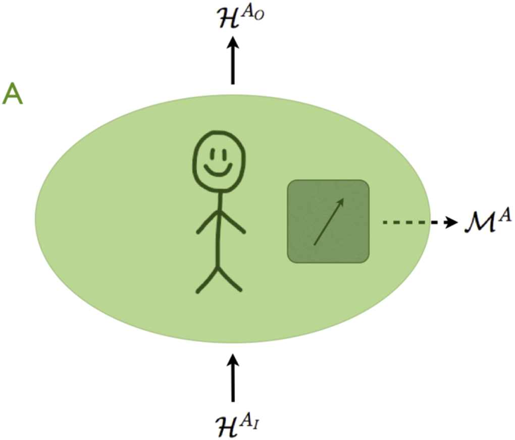
Formally, an event in region A is represented by a completely positive trace-non-increasing (CP) map ${{ \mathcal M }}^{A}:{A}_{I}\to {A}_{O}$, where input and output spaces are the spaces of linear operators over input and output Hilbert spaces of the local region, ${A}_{I}\equiv { \mathcal L }({{ \mathcal H }}^{{A}_{I}})$, ${A}_{O}\equiv { \mathcal L }({{ \mathcal H }}^{{A}_{O}})$ respectively (here identified with the corresponding matrix spaces) [36], see figure 2. We write ${L}^{A}:= { \mathcal L }({A}_{I},{A}_{O})$ for the set of linear maps from A_I to A_O. We denote the set of CP maps associated to each region, ${{\rm{CP}}}^{X}\subset {L}^{X}$.

Zoom In Zoom Out Reset image size

We demand complete positivity because in principle it should be possible to perform arbitrary quantum operations in the local region. This includes performing operations on a subsystem that is part of a larger system. Complete positivity means that, for arbitrary dimensions of an ancillary system $A^{\prime}$, the map ${{ \mathcal I }}^{A^{\prime} }\otimes {{ \mathcal M }}^{A}$ transforms positive operators into positive operators, where ${{ \mathcal I }}^{A^{\prime} }$ is the identity map on $A^{\prime}$. Trace non-increasing means that $\mathrm{Tr}{ \mathcal M }(\rho )\leqslant \mathrm{Tr}\rho$ for all operators ρ. A CP map can be decomposed as ${ \mathcal M }(\rho )={\sum }_{j=1}^{m}{K}_{j}\rho {K}_{j}^{\dagger }$, where the Kraus operators ${K}_{j}:{{ \mathcal H }}^{{A}_{I}}\to {{ \mathcal H }}^{{A}_{O}}$, j = 1, ..., m, satisfy ${\sum }_{j=1}^{m}{K}_{j}^{\dagger }{K}_{j}\leqslant {\mathbb{1}}$ for a trace non-increasing map [37, 38].

The context for each set of CP maps is now no longer a POVM but rather a quantum instrument [39]. An instrument thus represents the collection of all possible events that can be observed given a specific choice of local action. Given a local region A, an instrument is formally defined as a set ${{\mathfrak{I}}}^{A}$ of CP maps that sum up to a completely positive trace-preserving (CPTP) map:

$$\begin{eqnarray}&&\mathrm{Tr}\left[\displaystyle \sum _{{{ \mathcal M }}^{A}\in {{\mathfrak{I}}}^{A}}{{ \mathcal M }}^{A}(\rho )\right]=\mathrm{Tr}(\rho ).\end{eqnarray} \tag{ 4 }$$

We are now in a position to define the relevant frame function and derive the appropriate probability rule for this scenario. Just as the Born rule tells us how to calculate the probability of a particular outcome given the relevant measurement operator, the Quantum Process Rule should tell us how to assign a joint probability to each possible collection of local events given the relevant instruments. We assume 'instrument' non-contextuality, rather than 'measurement' non-contextuality. That is, the joint probability for a set of events, one for each region, is independent of the particular context (set of instruments) to which they belong, see figure 3.

Zoom In Zoom Out Reset image size

As for [30], the non-contextuality assumption is formalised by requiring that probabilities are given by a frame function. Each 'frame' is now a collection of instruments, one per region, rather than a single POVM.

Definition 1. A frame function, f, for a set of local non-intersecting regions X = A, B, C, ..., is defined by:

• 1.  
  f is a function from the Cartesian product of the set of CP maps associated to each region, ${{\rm{CP}}}^{X}\subset {L}^{X}$, to the unit interval:

  $$\begin{eqnarray}&&f:{{\rm{CP}}}^{A}\times {{\rm{CP}}}^{B}\times {{\rm{CP}}}^{C}...\,\to \,[0,1]\end{eqnarray} \tag{ 5 }$$
• 2.  
  f is normalised for all sets of CP maps, ${{ \mathcal M }}^{X}$, that form instruments ${{\mathfrak{I}}}^{X}$,

  $$\begin{eqnarray}&&\displaystyle \sum _{\begin{array}{c}{{ \mathcal M }}^{A}\in {{\mathfrak{I}}}^{A}\\ {{ \mathcal M }}^{B}\in {{\mathfrak{I}}}^{B}\\ {{ \mathcal M }}^{C}\in {{\mathfrak{I}}}^{C}\\ ...\end{array}}f({{ \mathcal M }}^{A},{{ \mathcal M }}^{B},{{ \mathcal M }}^{C},\,\mathrm{...})=1\end{eqnarray} \tag{ 6 }$$

We now show that this definition is sufficient to derive the new probability rule. As in [30] we first prove linearity of the frame function.

Theorem 1. The frame function f is a convex-multilinear functional on ${{\rm{CP}}}^{A}\times {{\rm{CP}}}^{B}\times {{\rm{CP}}}^{C}\times ...$

By convex-multilinear we mean:

$$\begin{eqnarray*}&&f[p{{ \mathcal M }}_{1}^{A}+(1-p){{ \mathcal M }}_{2}^{A},{{ \mathcal M }}^{B},{{ \mathcal M }}^{C},\,\mathrm{...}]\\ &&\quad =\,{pf}[{{ \mathcal M }}_{1}^{A},{{ \mathcal M }}^{B},{{ \mathcal M }}^{C},\,\mathrm{...}]+(1-p)f[{{ \mathcal M }}_{2}^{A},{{ \mathcal M }}^{B},{{ \mathcal M }}^{C},\,\mathrm{...}]\\ &&(0\leqslant p\leqslant 1)\end{eqnarray*}$$

and similarly for all other regions $B,C,\,...$

Proof. We fix instruments at all regions, except for region A, to be instruments with a single CPTP map each: ${\overline{{ \mathcal M }}}^{B},\,{\overline{{ \mathcal M }}}^{C},\,...$

Consider two instruments applied in region A:

$$\begin{eqnarray*}{{\mathfrak{I}}}_{1}^{A} & = & \{{{ \mathcal M }}_{1}^{A},\,{{ \mathcal M }}_{2}^{A},\,{{ \mathcal M }}_{3}^{A}\},\\ {{\mathfrak{I}}}_{2}^{A} & = & \{{{ \mathcal M }}_{1}^{A}+{{ \mathcal M }}_{2}^{A},\,{{ \mathcal M }}_{3}^{A}\}.\end{eqnarray*}$$

The frame function constraints imply:

$$\begin{eqnarray*}f[{{ \mathcal M }}_{1}^{A},\,{\overline{{ \mathcal M }}}^{B},\,\mathrm{...}]+f[{{ \mathcal M }}_{2}^{A},\,{\overline{{ \mathcal M }}}^{B},\mathrm{..}]+f[{{ \mathcal M }}_{3}^{A},\,{\overline{{ \mathcal M }}}^{B},\mathrm{..}] & = & 1\\ f[({{ \mathcal M }}_{1}^{A}+{{ \mathcal M }}_{2}^{A}),\,{\overline{{ \mathcal M }}}^{B},\,\mathrm{...}]+f[{{ \mathcal M }}_{3}^{A},\,{\overline{{ \mathcal M }}}^{B},\,\mathrm{...}] & = & 1.\end{eqnarray*}$$

Therefore

$$\begin{eqnarray*}&&f[{{ \mathcal M }}_{1}^{A},\,{\overline{{ \mathcal M }}}^{B},\,\mathrm{...}]+f[{{ \mathcal M }}_{2}^{A},\,{\overline{{ \mathcal M }}}^{B},\,\mathrm{..}]\\ &&\quad =\,f[({{ \mathcal M }}_{1}^{A}+{{ \mathcal M }}_{2}^{A}),\,{\overline{{ \mathcal M }}}^{B},\,\mathrm{...}]\end{eqnarray*}$$

and thus we have additivity for CP, trace non-increasing maps.

We next prove homogeneity of the frame function for the rational numbers between 0 and 1. Take two integers $1\leqslant n\leqslant m\in {\mathbb{N}}$, and a CP, trace-non-increasing map ${ \mathcal M }$. By converting multiplications by integers into sums, from additivity of the frame function we have:

$$\begin{eqnarray}\displaystyle \frac{n}{m}f({ \mathcal M }) & = & \displaystyle \frac{n}{m}f\left(\displaystyle \sum _{j=1}^{m}\displaystyle \frac{{ \mathcal M }}{m}\right)\\ & = & \displaystyle \frac{n}{m}\displaystyle \sum _{j=1}^{m}f\left(\displaystyle \frac{{ \mathcal M }}{m}\right)=\displaystyle \sum _{i=1}^{n}f\left(\displaystyle \frac{{ \mathcal M }}{m}\right)\\ & = & f\left(\displaystyle \sum _{i=1}^{n}\displaystyle \frac{1}{m}{ \mathcal M }\right)=f\left(\displaystyle \frac{n}{m}{ \mathcal M }\right).\end{eqnarray} \tag{ 7 }$$

Therefore, having additivity and homogeneity, we have proved the convex linearity of f for rational numbers between 0 and 1.

Convex linearity of the frame function on the real interval [0, 1] can be established using the 'squeeze theorem' of elementary calculus [40]. Define two sequences of positive rationals, $\{{a}_{n}\}$ increasing and $\{{b}_{n}\}$ decreasing with ${a}_{n}\lt {b}_{n}\leqslant 1$, that converge to the same real number c. Then, for any CP map ${{ \mathcal M }}^{A}$, the map ${{ \mathcal N }}_{n}^{A}:= (c-{a}_{n}){{ \mathcal M }}^{A}$ is also CP. Thus, fixing all maps in other regions to be CPTP, we have

$$\begin{eqnarray*}&&f(c{{ \mathcal M }}^{A},\,\mathrm{...})\\ &&\quad =\,f({a}_{n}{{ \mathcal M }}^{A},\,\mathrm{...})+f({{ \mathcal N }}_{n}^{A},\,\mathrm{...})\geqslant f({a}_{n}{{ \mathcal M }}^{A},\,\mathrm{...}).\end{eqnarray*}$$

Similarly, we have that $f(c{{ \mathcal M }}^{A},\,\mathrm{...})\leqslant f({b}_{n}{{ \mathcal M }}^{A},\,\mathrm{...})$. This implies

$$\begin{eqnarray}&&{a}_{n}f({{ \mathcal M }}^{A},\,\mathrm{...})\leqslant f(c{{ \mathcal M }}^{A},\,\mathrm{...})\leqslant {b}_{n}f({{ \mathcal M }}^{A},\,\mathrm{...}).\end{eqnarray} \tag{ 8 }$$

Because ${a}_{n}f({{ \mathcal M }}^{A},\,\mathrm{...})$ and ${b}_{n}f({{ \mathcal M }}^{A},\,\mathrm{...})$ both converge to ${cf}({{ \mathcal M }}^{A},\,\mathrm{...})$, equation (8) implies

$$\begin{eqnarray}&&f(c{{ \mathcal M }}^{A},\,\mathrm{...})={cf}({{ \mathcal M }}^{A},\,\mathrm{...})\end{eqnarray} \tag{ 9 }$$

by the 'squeeze theorem'.

We have thus proved that f is linear on CP^A and, with similar steps, linearity can be proved for CP^B, CP^C, ...which concludes the proof.□

Just as in ordinary quantum mechanics a state is defined as a linear functional over effects (POVM elements), we can define a multilinear functional over sets of events (CP maps) as a process, in accordance with the terminology of [20, 22, 41–48].

We next use the fact that a linear functional can be expressed by means of an inner product. This enables us to derive a new probability rule using our frame function, and also gives the appropriate form for the matrix representation of a process.

First consider that because each convex space CP^X contains a basis of the entire linear space L^X, X = A, B, ..., the frame function f can be extended by linearity to a multilinear function on the spaces L^A, L^B, L^C, ... Again by linear extension, this defines a unique linear function on the product space ${L}^{A}\otimes {L}^{B}\otimes {L}^{C}\otimes ...$

Next, it is easy to show that a natural inner product between any two linear maps ${{ \mathcal M }}^{A}$, ${{ \mathcal N }}^{A}$ ∈ L^A is defined as follows (see the appendix for details):

$$\begin{eqnarray}&&({{ \mathcal M }}^{A},{{ \mathcal N }}^{A}):= \displaystyle \sum _{\mu }\mathrm{Tr}[{{ \mathcal M }}^{A}{({\tau }_{\mu })}^{\dagger }{{ \mathcal N }}^{A}({\tau }_{\mu })],\end{eqnarray} \tag{ 10 }$$

where ${\{{\tau }_{\mu }\}}_{\mu =0}^{{d}^{2}-1}$ is a Hilbert–Schmidt basis for the d-dimensional input space: ${\tau }_{\mu }\in { \mathcal L }({{ \mathcal H }}^{{A}_{I}})$, ${\tau }_{\mu }={\tau }_{\mu }^{\dagger }$, $\mathrm{Tr}({\tau }_{\mu }{\tau }_{\nu })={\delta }_{\mu \nu }$.

One can also represent this inner product in a more convenient (and familiar) form by representing the CP maps associated to each region as Choi–Jamiolkowski (CJ) matrices [49, 50]. Recall, a CP map associated to a region A, where input and output spaces are the spaces of linear operators over input and output Hilbert spaces, ${A}_{I}\equiv { \mathcal L }({{ \mathcal H }}^{{A}_{I}})$, ${A}_{O}\equiv { \mathcal L }({{ \mathcal H }}^{{A}_{O}})$, respectively, can be represented as a matrix⁵ :

$$\begin{eqnarray}&&{M}^{A}={\displaystyle \sum }_{jl}{| l\rangle \langle j| }^{{A}_{I}}\otimes {[{ \mathcal M }{(| j\rangle \langle l| )}^{{A}_{O}}]}^{T},\end{eqnarray} \tag{ 11 }$$

where ^T denotes transposition in a chosen basis and ${\{| j\rangle \}}_{j=1}^{{d}_{{A}_{I}}}$ is an orthonormal basis in ${{ \mathcal H }}^{{A}_{I}}$. We show in the appendix that the inner product (10) can be expressed as

$$\begin{eqnarray}&&({{ \mathcal M }}^{A},{{ \mathcal N }}^{A})=\mathrm{Tr}({M}^{A\dagger }{N}^{A})\end{eqnarray} \tag{ 12 }$$

and it is independent of the choice of Hilbert–Schmidt basis.

This inner product determines an isomorphism between elements of ${L}^{A}\otimes {L}^{B}\otimes {L}^{C}\otimes ...$ and linear functionals on the same space. We can thus define a trace rule that allows one to determine the joint probability for a set of CP maps, one for each region:

$$\begin{eqnarray}&&f({{ \mathcal M }}^{A},{{ \mathcal M }}^{B}\,,...)\\ &&\quad =\,({{ \mathcal W }}_{f},{{ \mathcal M }}^{A}\otimes {{ \mathcal M }}^{B}\otimes ...)\\ &&\quad =\,\mathrm{Tr}[({M}^{A}\otimes {M}^{B}\otimes ...)\cdot {W}_{f}^{{AB}...}],\end{eqnarray} \tag{ 13 }$$

where ${{ \mathcal W }}_{f}\in {L}^{A}\otimes {L}^{B}\otimes {L}^{C}\otimes ...$ is the linear map that uniquely defines f and ${W}_{f}^{{AB}...}$ is its CJ representation, called the process matrix. (In the following, we will drop the subscript f.)

Positivity and normalisation of the frame function, equations (5) and (6) respectively, impose constraints on the operators W that define valid processes. The set of process matrices, together with the expression (13) for the frame function, defines the Quantum Process Rule. As discussed in [20], the set of matrices characterised by positivity, equation (5), is further restricted if one assumes that local operations can be extended to act on additional multipartite quantum states shared among the regions. The overall result can be summarised as follows:

Theorem 2. Given a set of regions $X=A,B,\,...$ where arbitrary quantum operations can be performed, any instrument non-contextual probability assignment, expressed through a frame function as per definition 1, must be given by the Quantum Process Rule, equation (13), where the process matrix $W$ satisfies the conditions

$$\begin{eqnarray}&&{\rm{Tr}}[({\bar{{\rm{M}}}}^{{\rm{A}}}\otimes {\bar{{\rm{M}}}}^{{\rm{B}}}\otimes ...)\cdot {{\rm{W}}}^{{\rm{AB}}...}]=1\end{eqnarray} \tag{ 14 }$$

$$\begin{eqnarray}&&\forall \,{\overline{M}}^{X}\,{\rm{s.t.}}\,{\rm{}}{\mathrm{Tr}}_{{X}_{O}}{\overline{M}}^{X}={{\mathbb{1}}}^{{X}_{I}}\end{eqnarray} \tag{ 15 }$$

and

$$\begin{eqnarray}&&\mathrm{Tr}[({M}^{A}\otimes {M}^{B}\otimes ...)\cdot {W}^{{AB}...}]\geqslant 0\\ &&\forall \,{M}^{X}\geqslant 0.\end{eqnarray} \tag{ 16 }$$

If one additionally assumes that each operation in region $X$ can be extended to act on an additional input space ${X}_{I}^{{\prime} }$, with an arbitary multipartite state ${\rho }^{{A}_{I}^{{\prime} }{B}_{I}^{{\prime} }...}$ shared across the regions, then the process matrix must be positive semidefinite, $W\geqslant 0$, a strictly stronger condition than equation (16).

Property (15) is the CJ representation of the trace-preserving condition; therefore, the normalisation constraint says that CPTP maps can be performed with unit probability. The resulting constraint on process matrices differs from the analogous one for density matrices, $\mathrm{Tr}\rho =1$. In addition to an analogous affine constraint, $\mathrm{Tr}W={d}_{O}$ with d_O the product of all output dimensions, W has to satisfy further linear constraints. We refer to appendix B of [42] for an explicit characterisation of such constraints.

Let us recapitulate the rationale so far: it was shown in [30] that if we accept the structure of quantum measurements, we can identify quantum probabilities as the most general non-contextual probability assignments. Whereas this approach only considers a single measurement/event—or at most measurements of separate quantum systems—in the quantum process approach outlined above we derive a general rule to assign joint probabilities to an arbitrary number of events. The ordinary Born rule is thus recovered from the general one in the case where a single region is considered—in which case instruments reduce to POVMs and process matrices reduce to density matrices [20].

We are in particular interested in the situation where two consecutive measurements are performed on a single quantum system. Gleason-type derivations of quantum probabilities do not tell us how to assign joint probabilities to two such events: one must introduce an additional ingredient—the state update rule. If the statistics for the first measurement are described by a density matrix ρ, and the first measurement is described by a CP map ${ \mathcal M }$, one calculates the probabilities for the second measurement, given the outcome of the first is known, by applying the Born rule to the updated state [51]

$$\begin{eqnarray}&&\rho \rightsquigarrow{\widetilde{\rho }}_{{ \mathcal M }}=\displaystyle \frac{{ \mathcal M }(\rho )}{\mathrm{Tr}{ \mathcal M }(\rho )}=\displaystyle \frac{{\displaystyle \sum }_{j=1}^{m}{K}_{j}\rho {K}_{j}^{\dagger }}{\mathrm{Tr}\phantom{\rule{}{1ex}}({\displaystyle \sum }_{j=1}^{m}{K}_{j}^{\dagger }{K}_{j}\rho \phantom{\rule{}{1ex}})}.\end{eqnarray} \tag{ 17 }$$

(Note that the update rule does not depend on the particular decomposition of ${ \mathcal M }$ into Kraus operators ${\{{K}_{j}\}}_{j=1}^{m}$.) In an operational perspective, rule (17) is seen as a quantum analogue of classical knowledge update. Within the quantum process framework, this is more than an analogy: the update rule is derived from the joint probability assignment.

To make the argument rigorous, we should remark again that the quantum frame function is not a normalised probability measure over the entire space of potential events. Formally, the frame function defines a parametrised probability for observing a CP map ${{ \mathcal M }}^{X}$ given an instrument ${{\mathfrak{I}}}^{X}$ in regions X = A, ...:

$$\begin{eqnarray}P({{ \mathcal M }}^{A},\,\mathrm{...}| {{\mathfrak{I}}}^{A},...) & = & f({{ \mathcal M }}^{A},\,\mathrm{...})\quad {\rm{if}}\,{\rm{}}{{ \mathcal M }}^{A}\in {{\mathfrak{I}}}^{A},\,\mathrm{...}\\ & = & 0\quad {\rm{otherwise.}}\end{eqnarray} \tag{ 18 }$$

(This defines a conditional probability if a marginal $P({{\mathfrak{I}}}^{A},\,\mathrm{...})$ is assigned.) Even though the inclusion of instruments is necessary to define (18) as a classical probability, we will omit them in the following for notational convenience.

Expression (18) defines an ordinary, classical probability measure, which lets us use all the machinery of classical probability theory. In particular, the conditional probability to observe ${{ \mathcal M }}^{B}$ in region B, given that ${{ \mathcal M }}^{A}$ is observed in region A, can be calculated from the joint probability distribution:

$$\begin{eqnarray}P({{ \mathcal M }}^{B}| {{ \mathcal M }}^{A}) & = & \displaystyle \frac{P({{ \mathcal M }}^{B},{{ \mathcal M }}^{A})}{P({{ \mathcal M }}^{A})}\\ & = & \displaystyle \frac{{\rm{Tr}}[({M}^{A}\otimes {M}^{B})\cdot W]}{{\displaystyle \sum }_{{M}^{B}\in {{\mathfrak{I}}}^{B}}{\rm{Tr}}[({M}^{A}\otimes {M}^{B})\cdot W]}\\ & = & {\rm{Tr}}({M}^{B}\,{\widetilde{W}}_{{M}^{A}}),\end{eqnarray} \tag{ 19 }$$

where we introduced the conditional process matrix [44]

$$\begin{eqnarray}&&{\widetilde{W}}_{{M}^{A}}:= \displaystyle \frac{{{\rm{Tr}}}_{{A}_{I}{A}_{O}}[({M}^{A}\otimes {{\mathbb{1}}}^{B})\cdot W]}{{\rm{Tr}}\left[\left({M}^{A}\otimes {\displaystyle \sum }_{{M}^{B}\in {{\mathfrak{I}}}^{B}}{M}^{B}\right)\cdot W\right]}.\end{eqnarray} \tag{ 20 }$$

Relevant to the ordinary state update rule is the case where A precedes temporally B, and the evolution between the two events is trivial. This scenario is described by the process matrix (see, e.g., [22])

$$\begin{eqnarray}&&W={\rho }^{{A}_{I}}\otimes {[[{\mathbb{1}}]]}^{{A}_{O}{B}_{I}}\otimes {{\mathbb{1}}}^{{B}_{O}},\end{eqnarray} \tag{ 21 }$$

$$\begin{eqnarray}&&{[[{\mathbb{1}}]]}^{{A}_{O}{B}_{I}}:= \displaystyle \sum _{{jl}}{| j\rangle \langle l| }^{{A}_{O}}\otimes {| j\rangle \langle l| }^{{B}_{I}},\end{eqnarray} \tag{ 22 }$$

where ρ is the density matrix describing the input state of region A. A straightforward calculation shows that, in this case, the conditional process matrix reduces to

$$\begin{eqnarray}&&{\widetilde{W}}_{{M}^{A}}={\left[\displaystyle \frac{{{ \mathcal M }}^{A}(\rho )}{\mathrm{Tr}{{ \mathcal M }}^{A}(\rho )}\right]}^{{B}_{I}}\,\otimes {{\mathbb{1}}}^{{B}_{O}}\equiv {\widetilde{\rho }}_{{{ \mathcal M }}^{A}}\otimes {{\mathbb{1}}}^{{B}_{O}},\end{eqnarray} \tag{ 23 }$$

which is the process matrix description of region B receiving a state described by the density matrix ${\widetilde{\rho }}_{{{ \mathcal M }}^{A}}$.

Some clarification at this point might be helpful regarding the distinction between probabilistic conditioning and knowledge update (see, e.g., [52] for a more detailed discussion). In classical probability theory, the rules for probabilistic conditioning simply follow from the axioms of the theory. These axioms can be assumed, as in Kolmogorov's approach, or derived from requirements on how one should consistently assign degrees of belief, for example through Dutch book arguments [53] or theorems like that of Savage [54]. A consequence of probabilistic conditioning is Bayes' theorem for inverting conditional probabilities:

$$\begin{eqnarray*}&&P(A| B)=P(B| A)\displaystyle \frac{P(A)}{P(B)}.\end{eqnarray*}$$

Importantly, this rule does not involve updating knowledge given new information: all information is contained in the joint probability P(A, B), which is unchanged by the application of the theorem.

Knowledge update, on the other hand, refers to the process of updating one's belief following the acquisition of new data. This process is not encoded in the axioms of probability theory and requires extra assumptions. For example, if one assumes that all data values that were not observed can be discarded, one arrives at Bayes rule:

$$\begin{eqnarray*}&&{P}_{{\rm{new}}}(A)={P}_{{\rm{old}}}(A| B=b),\end{eqnarray*}$$

where b is the observed value of the variable B. Implicit in this rule is the counterfactual assumption that values that are not observed are known to be false. Thus, applying Bayes theorem, one arrives at the standard form for Bayes updating:

$$\begin{eqnarray*}&&{P}_{{\rm{new}}}(A)={P}_{{\rm{old}}}(A)\displaystyle \frac{{P}_{{\rm{old}}}(B=b| A)}{{P}_{{\rm{old}}}(B=b)}.\end{eqnarray*}$$

In the quantum case, such counterfactual assumptions are known to be problematic [55]⁶ . In our approach, no such assumption is necessary, because the primitive object is the joint probability. From this perspective, the 'state update' rule is not an update at all, but rather an application of probabilistic conditioning. This insight distinguishes this approach from other attempts to leverage Bayesian arguments to justify an informational interpretation of quantum theory [21, 23].