


Abstract
Understanding what distinguishes quantum mechanics from classical mechanics is crucial for quantum information processing applications. In this work, we consider two notions of non-classicality for quantum systems, negativity of the Wigner function and contextuality for Pauli measurements. We prove that these two notions are equivalent for multi-qudit systems with odd local dimension. For a single qudit, the equivalence breaks down. We show that there exist single qudit states that admit a non-contextual hidden variable model description and whose Wigner functions are negative.
Export citation and abstract BibTeX RIS
1. Introduction
Understanding what distinguishes quantum mechanics from classical mechanics and probabilistic models is a central question of physics. Besides its foundamental aspects, this question is crucial for quantum information processing applications since the features that set quantum and classical mechanics appart are precisely the properties that we must exploit in order to obtain a quantum superiority for certain tasks [1–20]. In the present work, we compare two notions of non-classicality: contextuality [21–27] and negativity of the Wigner function [28–30].
The Wigner function shares several properties of probability distributions with the difference that it can take negative values. This phenomenon is generally considered as an indicator of non-classicality of quantum states [31–36] (see also the discussion in [37]).
The ressemblance between contextuality and negativity was exploited by Spekkens who generalized these two notions in order to prove that they coincide [38]. However, this result remains difficult to apply, since a large number of Wigner functions must be probed to identify contextuality. Howard et al [18] showed that, if one restricts to a particular class of measurements, namely Pauli measurements, one can select a particular Wigner function which allows by itself to characterize contextuality in the traditional Kochen–Specker sense [22]. They proved that contextuality for stabilizer measurements and negativity of Gross' Wigner function [30] coincide for quopits, i.e. odd prime dimensional qudits. Namely, they showed that a single quopit state ρ has a negative Wigner function if and only if its tensor product with any other single-quopit state violates a two-quopit non-contextuality inequality.
In the present work, we establish the equivalence between contextuality for stabilizer measurements and negativity of Gross' Wigner function [30] for any multi-qudit state with odd local dimension. Such a neat equivalence between these features introduced in different fields is quite unexpected. Indeed, while contextuality is grounded in the foundations of quantum physics, Wigner functions originate from quantum optics. In addition, our proof of this equivalence is much more straightforward. Indeed, we directly compute the value of the Wigner function in terms of the hidden variable model (HVM) and we observe that if the HVM is non-contextual then the Wigner function is non-negative. Howard et al required a two-qudit experiment to demonstrate contextuality of a single qudit state. We elucidate this by showing explicitly that in a single qudit experiment, the equivalence between contextuality and negativity does not hold. We show this by constructing quantum states that admit a non-contextual HVM (NCHVM) description although their Wigner functions take negative values.
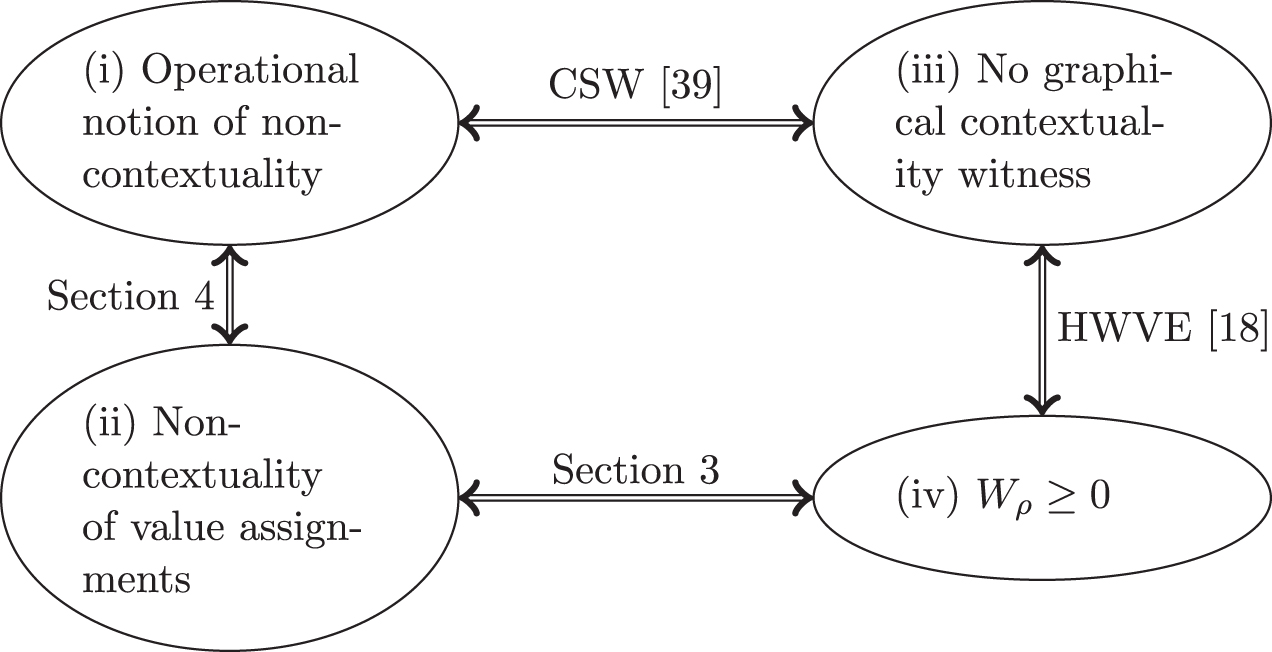
Our proof of this equivalence relies on the choice of a simple definition of contextuality based on value assignments introduced in the work of Kochen and Specker [22], whereas the work of Howard et al is based on the graphical formalism of Cabello et al [39]. The relations between these different notions of non-classicality are depicted in figure 1. Following [22–24], we consider only contextuality of stabilizer measurements and HVMs are assumed to be deterministic. This last assumption is also present in the graphical formalism of Cabello et al [39] and in the work of Howard et al [18]. Our argument does not apply to the generalized notion of HVMs considered for instance by Spekkens [38, 40].

Figure 1. Relation between different notions of non-classicality. The equivalence HWVE [18] is only proven for product states when n = 2 and d is an odd prime number.
Download figure:
Standard image High-resolution imageOur work clarifies the relationship between discrete Wigner function and stabilizer contextuality for odd-dimensional qudits. It cannot be extended to systems of qubits due to the presence of state-independent contextuality [23–25]. In addition, no qubit Wigner function that satisfies all the properties of Gross' qudit Wigner function seems to exist [41–43].
This article is organized as follows. The necessary stabilizer formalism is recalled in section 2. Section 3 introduces a notion contextuality based on value assignment and a proof of the equivalence between this notion and the negativity of Gross' discrete Wigner function, i.e. (ii) ⇔ (iv). The purpose of section 4 is to prove the equivalence between the two notions of contextuality (i) and (ii), completing the square in figure 1.
2. Background on the stabilizer formalism
In what follows, we consider the Hilbert space  , where d is an odd integer and n is a non-negative integer. We consider an orthonormal basis
  of
of  . The n-fold tensor products of these vectors provide an orthonormal basis
  of the Hilbert space
  indexed by
  . This section recalls standard tools of the stabilizer formalism for qudits [44].
The space  that is called the phase space and will be used to index generalized Pauli operators acting on
  . Vectors in V are denoted
  , where both
  and
and  live in
  . The space
  is equipped with the standard inner product
  for all
  , whereas the phase space V is equipped with the symplectic inner product defined by

where  and
and  .
.
Pauli matrices can be generalized to obtain matrices acting on  as follows. Let ω be the dth root of unity,
  . The generalized Pauli matrices X and Z are defined by

for all  , where the addition of basis labels is considered modulo d. Tensor products of these matrices are denoted
  and
and  where
where  . They satisfy
 .
.
Generalized Pauli operators acting on this Hilbert space  are of the form
  where
where  , and
, and  . Just as qubit Pauli operators, they form a group. We fix the phase of
  to be
to be  . Recall that, since d is an odd integer,
  exists in
  and the term
  is a well defined element of
  . This defines Heisenberg–Weyl operators

for all  . This choice is well suited to describe measurement outcomes since
 ![${T}_{{\bf{u}}}{T}_{{\bf{v}}}={\omega }^{[{\bf{u}},{\bf{v}}]/2}{T}_{{\bf{u}}+{\bf{v}}}$](https://content.cld.iop.org/journals/1367-2630/19/12/123024/revision1/njpaa8fe3ieqn37.gif) , in particular two operators
, in particular two operators  and
and  can be measured simultaneously if and only if
 ![$[{\bf{u}},{\bf{v}}]=0$](https://content.cld.iop.org/journals/1367-2630/19/12/123024/revision1/njpaa8fe3ieqn40.gif) , which implies
, which implies  . Their commutation relation depends on the symplectic inner product as follows
 ![${T}_{{\bf{u}}}{T}_{{\bf{v}}}={\omega }^{[{\bf{u}},{\bf{v}}]}{T}_{{\bf{v}}}{T}_{{\bf{u}}}$](https://content.cld.iop.org/journals/1367-2630/19/12/123024/revision1/njpaa8fe3ieqn42.gif) . These operators satisfy
. These operators satisfy  which proves that their eigenvalues belong to the group
  of dth roots of unity.
Measuring a family of m mutually commuting operators  returns the outcome
  with probability
  , where
  is the projector onto the common eigenspace of the operators
  with respective eigenvalue
  . When no confusion is possible, this projector is simply denoted
  . Such a subset C of mutually commuting operators is called a context. The largest possible size of a context is dn, which means that
  . The set of all the contexts is denoted
  . For a single operator
  , we have
  , by definition of these projectors. Moreover,
  can be obtained from the operator
  as
as

Indeed, one can check that if  is an eigenvector of
  with eigenvalue
  , we have

 In order to generalize equation (2) to a family
  of operators, introduce the
  -linear subspace
  of V generated by the vectors
  . Any measurement outcome
  induces a
  -linear form
  defined by
  where
where  for all
  . This map
  parametrizes the group generated by the operators
  as follows
  . The projector
  can be written

This expression can be deduced from equation (2) by writing  as the product
  . The image of the projector (3) is a stabilizer code [44].
3. Contextuality of value assignments and negativity
In this section, we prove that the notion of non-contextuality based on the existence of non-contextual value assignments [22–25] is equivalent to the non-negativity of the discrete Wigner function. A special case of this equivalence was proven by Howard et al [18] in odd prime dimension. We propose a simple proof of this result which allows us to generalize this equivalence to any system of multiple qudits and to any odd local dimension.
Recall that contextuality refers to the fact that measurement outcomes cannot be described in a deterministic way [22]. One cannot associate a fixed outcome  with each observable A in such a way that this value is simply revealed after measurement. The algebraic relations between compatible observables must be satisfied by outcomes as well, making the existence of such pre-existing outcomes impossible. For instance, given two commuting operators A and B, the three observables A, B and C = AB can be measured simultaneously and the values
  and
and  associated with these operators must satisfy
  . No value assignment satisfying all these algebraic constraints exists in general.
The Wigner function of a state is a description of this state that was introduced in quantum optics in order to identify states with a classical behavior. Quantum states with a non-negative Wigner function are considered as quasi-classical states. The non-negativity of the Wigner function allows to describe the statistics of the outcomes of a large class of measurements in a classical way. The success of this representation motivated its generalization to finite dimensional Hilbert spaces, called discrete Wigner function. Different generalizations have been considered and finding a finite-dimensional Wigner representation that behaves as nicely as its original infinite-dimensional version [28] of use in quantum optics is a non-trivial question. The qubit case illustrates the difficulty of this task [41, 42]. In this work, we restrict ourselves to systems of qudits with odd local dimension and we consider Gross' discrete Wigner function which encloses most of the features of its quantum optics counterpart [30].
3.1. Value assignments are characters in odd local dimension
In this definition, the HVM associates a deterministic eigenvalue  with each operator
  . Measurements only reveal these pre-existing values that are independent on other compatible measurements being performed. Formally, non-contextual value assignments are defined as follows.
Definition 1. Let ρ be a density matrix over  . A set of NC value assignments for the state
  is a triple
  where S is a finite set,
  is a probability distribution over
  and
and  is a collection of maps
  , for each
  , such that
- 1.for all
![${\bf{u}},{\bf{v}}\in V,[{\bf{u}},{\bf{v}}]=0$](data:image/png;base64,iVBORw0KGgoAAAANSUhEUgAAAAEAAAABCAQAAAC1HAwCAAAAC0lEQVR42mNkYAAAAAYAAjCB0C8AAAAASUVORK5CYII=) implies ,
implies , - 2.for all,
![${\bf{u}},{\bf{v}}\in V,[{\bf{u}},{\bf{v}}]=0$](https://content.cld.iop.org/journals/1367-2630/19/12/123024/revision1/njpaa8fe3ieqn94.gif)


This definition corresponds to the notion of value assignment introduced by Kochen and Specker [22] restricted to measurements associated with Heisenberg–Weyl operators. The set S represents the hidden variable states or ontic states. Without loss of generality, one can assume that the value assignment associated with distinct states  are distinct. Then, S is necessarily a finite set since there is only a finite number of distinct maps
  from V to Ud. A map
  which satisfies
  for all
  such that
 ![$[{\bf{u}},{\bf{v}}]=0$](https://content.cld.iop.org/journals/1367-2630/19/12/123024/revision1/njpaa8fe3ieqn103.gif) , is called a value assignment. Recall that the value
, is called a value assignment. Recall that the value  is associated with the operator
  defined in equation (1). With this phase convention, a value assignment is defined in such a way that the value of the product
  of two compatible operators is the products of their values. As we will see later, multiplicativity of
  whenever
 ![$[{\bf{u}},{\bf{v}}]=0$](https://content.cld.iop.org/journals/1367-2630/19/12/123024/revision1/njpaa8fe3ieqn108.gif) is the non-contextuality assumption whereas the condition
is the non-contextuality assumption whereas the condition  ensures that this triple is sufficient to recover the prediction of quantum mechanics for the measurement of
  .
.
A value assignment is a map  that satisfies the constraint
  , for all pairs of vectors such that
 ![$[{\bf{u}},{\bf{v}}]=0$](https://content.cld.iop.org/journals/1367-2630/19/12/123024/revision1/njpaa8fe3ieqn113.gif) . This enourages us to consider the characters of V. Recall that a character of V is defined to be group morhism from V to the multiplicative group
. This enourages us to consider the characters of V. Recall that a character of V is defined to be group morhism from V to the multiplicative group  . In other words, it is a map
  that satisfies the constraint
  for all
  . There exist
  characters of V and they are of the form
 ![${\lambda }_{{\bf{a}}}({\bf{u}})={\omega }^{[{\bf{a}},{\bf{u}}]}$](https://content.cld.iop.org/journals/1367-2630/19/12/123024/revision1/njpaa8fe3ieqn119.gif) for some
for some  . These d2n characters provides d2n value assignments. Conversely, any value assignment
  coincindes with a character of V over any isotropic subspace. However, nothing in definition 1 guarantees that these assignments are actually characters of V. The next lemma proves this property. As a consequence, the only consistent value assignments of the HVM are given by the d2n characters of V.
Lemma 1. For any odd integer  and for any integer
  , value assignments
  are characters of
  .
.
Proof. To make the proof easier to follow, we regard λ as a map from V to  (through the group isomorphism between Ud and
  ) and we use the additive notation
  instead of
  in
in  . We already know that
  whenever
 ![$[{\bf{u}},{\bf{v}}]=0$](https://content.cld.iop.org/journals/1367-2630/19/12/123024/revision1/njpaa8fe3ieqn132.gif) . In particular for all
. In particular for all  and for all
  we have
  .
.
Consider the canonical basis of  that we denote
  . Clearly,
 ![$[{{\bf{e}}}_{{\bf{i}}},{{\bf{f}}}_{{\bf{i}}}]=1$](https://content.cld.iop.org/journals/1367-2630/19/12/123024/revision1/njpaa8fe3ieqn138.gif) and the planes
and the planes  are pairwise orthogonal with respect to the symplectic inner product for all
  . The orthogonality between these planes allows us to write

for all  . It remains to prove that the restriction of λ to any plane
  is additive.
We will use a second plane  with
with  (which exists only when
  ). Denote
  and
and  and define
  and
and  so that
 ![$[{\bf{u}},{\bf{v}}]=[{\bf{u}}^{\prime} ,{\bf{v}}^{\prime} ]$](https://content.cld.iop.org/journals/1367-2630/19/12/123024/revision1/njpaa8fe3ieqn150.gif) . To conclude it suffices to prove that
. To conclude it suffices to prove that  . Write

This decomposition is chosen in such a way that  and
and  are orthogonal:

We will also use the orthogonality relations ![$[{\bf{u}}\pm {\bf{v}}^{\prime} ,{\bf{v}}\pm {\bf{u}}^{\prime} ]=0$](https://content.cld.iop.org/journals/1367-2630/19/12/123024/revision1/njpaa8fe3ieqn154.gif) and between the planes
and between the planes  and Pj. We obtain

This proves that λ is a character.□
3.2. Discrete Wigner functions
The purpose of this section is to recall that a set of NC value assignments can be derived from a discrete Wigner function of a state whenever this function is non-negative [18].
Quantum states are generally represented by their density matrix ρ. The Wigner function Wρ of a state ρ is an alternative description of the state ρ. This representation is sometimes more convenient than the density matrix. Wigner functions have been introduced in quantum optics [28] and the negativity of the Wigner function of a state is regarded as an indicator of non-classicality of this quantum state. In the present work, we consider their finite dimensional generalization which is called discrete Wigner function [7, 29].
We focus on Gross' discrete Wigner function [30]  defined by
  where
where ![${A}_{{\bf{u}}}={d}^{-n}{\sum }_{{\bf{v}}\in V}{\omega }^{[{\bf{u}},{\bf{v}}]}{T}_{{\bf{v}}}$](https://content.cld.iop.org/journals/1367-2630/19/12/123024/revision1/njpaa8fe3ieqn158.gif) . The operators
. The operators  are Hermitian. The family
  is an orthonormal basis of the space of
  -matrices equipped with the inner product
  . The values
  for
for  are simply the coefficients of the decomposition of the matrix ρ in this basis:

This proves that the Wigner function Wρ fully describes the state ρ.
In order to describe measurement outcomes, the Wigner representation can be extended to POVM elements  . The Wigner function of a POVM element Es is defined to be
  This definition is chosen in such a way that the probability
  of the outcome s is given in terms of the Wigner functions Wρ and
  by
by

This expression is obtained by replacing ρ by its decomposition (4).
Consider for instance the measurement of an operator  . It corresponds to the POVM elements
  . Calculating the value of the Wigner function of the POVM element
  , we find
 ![${W}_{{{\rm{\Pi }}}_{{\bf{a}}}^{s}}({\bf{u}})={\delta }_{[{\bf{a}},{\bf{u}}],s},$](https://content.cld.iop.org/journals/1367-2630/19/12/123024/revision1/njpaa8fe3ieqn172.gif) and injecting this in equation (5) yields
and injecting this in equation (5) yields ![$\mathrm{Tr}({{\rm{\Pi }}}_{{\bf{a}}}^{s}\rho )={\sum }_{{\bf{u}}\in V}{\delta }_{[{\bf{a}},{\bf{u}}],s}{W}_{\rho }({\bf{u}}).$](https://content.cld.iop.org/journals/1367-2630/19/12/123024/revision1/njpaa8fe3ieqn173.gif) Using the decomposition of
Using the decomposition of  as a sum of projectors, this provides the expectation of
  .
.
Lemma 2. For all Heisenberg–Weyl operators  given in equation (1), it holds that

Comparing lemma 2 with definition 1, we see that the triple  is a set of NC value assignments for
 ![${\lambda }_{{\bf{u}}}({\bf{a}})={\omega }^{[{\bf{a}},{\bf{u}}]}$](https://content.cld.iop.org/journals/1367-2630/19/12/123024/revision1/njpaa8fe3ieqn178.gif) whenever the Wigner function of the state ρ is non-negative. Note that all characters of V can be written as
whenever the Wigner function of the state ρ is non-negative. Note that all characters of V can be written as ![${{\omega }}^{[\cdot ,{\bf{u}}]}$](https://content.cld.iop.org/journals/1367-2630/19/12/123024/revision1/njpaa8fe3ieqn179.gif) for some
for some  .
.
3.3. Equivalence between NC value assignments and non-negativity
The previous section shows that non-negativity of Wρ implies the existence of a set of NC value assignments for the state ρ. We now prove the converse statement.
Proposition 1. Let  and let
  be a n-qudits state of odd local dimension
  . If ρ admits a set of NC value assignments then
  .
.
Proof. Given a set of NC value assignments, let us compute the value of the Wigner function of ρ to prove that it is non-negative. We have

The fact that such a sum is positive or even real is not clear. However, lemma 1 shows that ![${\omega }^{[{\bf{u}},\cdot ]}{\lambda }_{\nu }(\cdot )$](https://content.cld.iop.org/journals/1367-2630/19/12/123024/revision1/njpaa8fe3ieqn185.gif) , which is a product of two characters, is also a character. Hence, any sum
, which is a product of two characters, is also a character. Hence, any sum ![${\sum }_{{\bf{v}}\in V}{\omega }^{[{\bf{u}},{\bf{v}}]}{\lambda }_{\nu }({\bf{v}})$](https://content.cld.iop.org/journals/1367-2630/19/12/123024/revision1/njpaa8fe3ieqn186.gif) is either 0 or d2n [45]. Since
is either 0 or d2n [45]. Since  , this proves that
  . □
. □
Actually the HVM derived from the discrete Wigner function is essentially unique. The following corollary shows that the distribution qρ of any set of NC value assignments can be identified with the Wigner function distribution Wρ over V.
Corollary 1. Let  and let
  be a n-qudits state of odd local dimension
  . If
. If  is a NC set of value assignments for ρ then there exists a bijective map
  such that

for all  .
.
Proof. Let us refine the argument of the proof of proposition 1. By lemma 1 and since value assignments corresponding to distinct states of S are assumed to be different, there exists an injective map  such that
 ![${\lambda }_{\nu }={\omega }^{[\phi (\nu ),\cdot ]}$](https://content.cld.iop.org/journals/1367-2630/19/12/123024/revision1/njpaa8fe3ieqn196.gif) . Without loss of generality, we can assume that ϕ is sujective by adding extra elements to S corresponding to the missing characters of V. For these new elements
. Without loss of generality, we can assume that ϕ is sujective by adding extra elements to S corresponding to the missing characters of V. For these new elements  , we simply set
  to preserve the prediction of the triple
  . With this notation, the expression of
  obtained in the previous proof becomes

For all vectors  , there exists a unique state
  such that
  . Denote by
  this state. Then, equation (6) becomes
  To conclude the proof, note that the map
  is invertible, by bijectivity of ϕ. Its inverse is the map σ of the corollary. □
3.4. The single qudit case
This section shows that the previous equivalence breaks down for single qudits.
Lemma 1 breaks down for n = 1. For instance, for a prime dimension d, there exists  value assignments while there is only d2 characters. Let us prove this property. By straightforward calculation we can check that two non-unit Pauli operators
  and
and  commute if and only if they are integer powers of one another. Therefore, each maximal context consists of a picked operator and its powers. Each non-unit observable thus appears in a single maximal context, and there are
  non-unit operators
  in each maximal context. The total number of non-unit Pauli operator is
  . Therefore, there are
  contexts. In each context, we can freely choose the value of one non-unit Pauli observable, and the other values in the context then follow. There are thus d choices per context, and the total number of value assignments is
  .
.
Breakdown of proposition 1 for n = 1 and d = 3. We consider the case of a single qutrit. Our strategy is to show that there is a valid quantum state that admits a set of NC value assignments, whose Wigner function is negative. To this end, we loop through all 81 consistent value assignments λ, and construct the density matrix  and Wigner function Wλ corresponding to each value assignment λ. The density matrix
  is given by

 reproduces the measurement statistics of the value assignment λ, i.e. in the measurement of Ta, the outcome
  is certain. Further,
  is Hermitian and has unit trace, but is in general not positive semidefinite.
To mitigate the latter shortcoming, we add an admixture of the completely mixed state to  , with increasing probability p,

We check whether the resulting state  becomes positive semidefinite before the corresponding Wigner function
  becomes positive, where
  denotes the constant Wigner function taking the value 1.
Denote the smallest eigenvalue of  by
by  , and the height of the deepest valley of Wλ by wλ. Because of the special form of the admixture, the smallest eigenvalue
  of
of  and the height
  of the deepest valley of
  are
are

Therefore, there is a region of p for which  is positive semidefinite while
  if and only if

Checking all 81 value assignments, we find that there are two cases.
Case I: value assignments that are characters of V (occurs 9 times).

The condition equation (7) is not satisfied, as expected for linear value assignments.
Case II: value assignments that are not characters of V (occurs 72 times).

The condition equation (7) is satisfied, and we thus know that there are positive semidefinite density matrices with negative Wigner functions. (The value of  above is minus the golden ratio.)
It remains to show that the density matrices  discussed in Case II have a representation in terms of NC value assignments. To this end, note that each
  has an NC value assignments representation, namely the probability distribution peaked at the assignment λ. The completely mixed state
  also has a NC value assignments description, namely it is the equal mixture of all value assignments that are characters of V. Hence, the probabilistic mixture of these two density matrices also is represented by a set of NC value assignments.
To summarize, we have shown that there are well-defined quantum states whose Wigner function is negative but which have an NCHVM description. These states are counterexamples to an extension of proposition 1 to n = 1. Our argument is presented for a qutrit but we believe that such single qudit states exist for all odd dimensions. We leave the general case as an open question. More generally, it would be interesting to provide a simple characterization of the single qudit states that admit a set of NC value assignments.
In [18], the equivalence between Wigner function negativity and contextuality is established for single qudit states, and the question arises whether their result and the above argument are in contradiction. This is not the case. The construction of [18] uses an auxiliary qudit that can be in any state σ, for instance the completely mixed state. The desired equivalence between Wigner function negativity and contextuality is established for one qudit states ρ by considering the tensor product state  on the contextuality side. Since σ is merely a by-stander, Howard et al count the setting as n = 1. By our counting, since the involved observables act on two qudits, the setting is n = 2. There is thus no contradiction between the result of [18] and the above argument that proposition 1 does not extend to n = 1.
4. Operational definition of non-contextuality
Our proof of the equivalence between non-contextuality and non-negativity of the Wigner function relies on the choice of a simple definition of contextuality (definition 1). The purpose of this section is to prove that, although simple, this definition is sufficient to capture the same notion of contextuality as the one considered in previous work [38, 40]. Namely, we prove that the notion of NC value assignments is equivalent to the operational definition of contextuality given below, inspired by the work of Spekkens with the restriction to deterministic models. All the results of this section are true for both multi-qudit systems and single qudit systems. They also remain valid for even local dimension d.
4.1. Deterministic hidden variable model
The role of a HVM is to describe the outcome distribution of Pauli measurements for a state ρ. In what follows, an ordered family of commuting operators  is called a context. This guarantees that they can be measured simultaneously. We denote by
  the set of all the contexts, that is of all ordered tuples of commuting Heisenberg–Weyl operators Tu.
The HVM considered in definition 1 is designed to predict the expectation of single Pauli operators. We now consider a framework which is a priori more general. The HVM is required to predict the outcome distribution of the measurement of any Pauli context  .
.
Definition 2. A HVM for a state  is defined to be a triple
  such that S is a set,
  is a distribution over
  and
and  is a family of conditional probability distributions
  over the possible outcome
  for any context
  and for any state
  . We require that the prediction of the HVM matches the quantum mechanical value, i.e.

for every context  and for every outcome
  .
.
The set S is the set of states of the HVM. Note that this set is not a priori the same as the set used in definition 1. We understand the probability  as the probability that the system is in the state
  . As suggested by the notation, the probability
  can be interpreted as the probability of an outcome
  when measuring the operators of the context C and when the system is in the state ν of the HVM. It is then natural to define the prediction of the HVM as in equation (8).
In the present work, we consider HVM that are deterministic in the following sense. We can associate a fixed measurement outcome  with each state ν of the model. In other words, conditional probabilities
  are delta functions.
Definition 3. A HVM  is said to be deterministic if conditional distributions
  are all delta functions, i.e. for all
  and for all outcome
  , we have
  for some map
  that associates a value
  with each context.
We often denote such a HVM by the triple  . When C contains m operators, both
  and
and  are m-tuples. If
  , then
  is the product of the delta functions
  .
.
4.2. Operational definition of non-contextuality
Within our formalism restricted to measurement of Pauli operators  , there exist different ways to realize a measurement. The operational notion of contextuality refers to the fact that the conditional distribution of outcomes in the HVM may depend on the way the measurement is implemented [40]. This section presents a formal definition of this notion.
To illustrate what should be the right definition of an implementation, we start with some examples. We can measure the operators of a context  and return the corresponding outcome
  . This realizes the measurement defined by the family of orthogonal projectors
  for
for  . Different contexts C may produce the same family of projectors, that is the same measurement. For instance, the 2-qudit measurement defined by the projectors
  indexed by
  , can be implemented via the contexts
  or alternatively via
  .
.
We can also measure of a family of operators but read only a subset of the outcomes or even of function of the outcomes. Such a classical postprocessing extends the set of projectors that can be reached. For instance, for  consider a pair of projectors
  . This measurement is realized by measuring
  and returning 0 if the outcome is 0 and returning 1 for all other outcomes
  . To provide an example with a less trivial postprocessing consider the measurement
  with outcome
  , for
, for  such that
 ![$[{\bf{u}},{\bf{v}}]=0$](https://content.cld.iop.org/journals/1367-2630/19/12/123024/revision1/njpaa8fe3ieqn287.gif) . We can realize this measurement by measuring the pair
. We can realize this measurement by measuring the pair  and by returning only the sum
  of the two outcomes.
These examples motivate our definition of an implementation of a measurement. Consider a measurement defined by a family of stabilizer projectors  , that sum up to identity, indexed by the elements of a finite set O.
Definition 4. An implementation of a measurement  , is defined to be a pair
  where
where  and
and  is a surjective postprocessing map such that

for all  .
.
Neither the choice of the context C nor the corresponding map  is unique. The postprocessing map is assumed to be surjective only to ensure that all the projectors of the family
  are reached.
Let  be a HVM describing measurement outcomes for a state ρ. Consider an implementation
  of a measurement
  . By definition of the projectors
  , the HVM predicts that the outcome
  occurs with probability

when the system is in position ν. Quantum mechanics predicts that the distribution of the outcome of a measurement only depends on the projectors  and not on the implementation. That means that for any two implementations
  and
and  of a measurement
  , we have

However, nothing in definition 2 requires that the probabilities  and
and  coincide for all
  . This assumption is a notion of non-contextuality. It leads to the following definition of a NCHVM. This definition is based on the work of Spekkens [40] with the restriction to deterministic models and to systems of qudits. Spekkens approach differs also in the fact that it does not refer to the internal structure of quantum mechanics at all. The relationship between Spekkens' form of contextuality and Kochen–Specker contextuality is examined here [46].
Definition 5. A HVM  is said to be non-contextual if for all implementations
  of a measurement
  , for all
  , the conditional probability
  depends only on the projector
  and not on the implementation
  .
.
For instance, we saw that the measurement  can be implemented by
  with a trivial map
  but also using
  with the postprocessing map
  . For a non-contextual model, the corresponding conditional probabilities
  and
and  coincide for all states ν of the HVM. In this example, we have
  .
.
4.3. Equivalence of the two definitions of non-contextuality
In this section we prove that the existence of a NCHMV as given in definition 5 and the existence of a set of NC value assignments as in definition 1 are two equivalent notions of non-contextuality. This is the equivalence (i)  (ii) in figure 1.
The following proposition shows that the implication (ii)  (i) holds.
Proposition 2. Let  be a n-qudit system with
  and
and  . If
. If  be a set of NC value assignments, then
  defines a deterministic NCHVM where p is defined by

for all  .
.
The notations  and
and  used in equation (9) were introduced in equation (3). Recall that, by deterministic, we mean
  .
.
Proof. First, let us prove that the HVM  defined in this proposition produces the same predictions as quantum mechanics. By equation (3), the probability of an outcome
  when measuring
  is given by

Replacing  by its value in terms of the value assignments, we obtain

This proves that the HVM  defined by equation (9) reproduces the quantum mechanical predictions.
It is deterministic since the sum  , which is the sum of the values of a character, is either 0 or
  , implying that
  . This HVM is also non-contextual. Indeed, conditional probabilities are defined in such a way that they do not depend on the particular choice of generators
  for the subspace
  , that is they do not depend on the context.□
We now prove the converse statement. Together with the non-contextuality assumption, determinism of the HVM yields extra compatibility contraints on the functions  . The following proposition proves that
  is completely determined by its value
  over single operator contexts
  . We shorten the notation
  by
by  . Moreover, we show that
  is additive when
 ![$[{\bf{u}},{\bf{v}}]=0$](https://content.cld.iop.org/journals/1367-2630/19/12/123024/revision1/njpaa8fe3ieqn353.gif) . Then, we will prove that we can construct a set of NC value assignments from the maps
. Then, we will prove that we can construct a set of NC value assignments from the maps  .
.
Proposition 3. Let  be a n-qudit system with
  and
and  . If
. If  is a deterministic NCHVM then,
- for all contexts , we have
- if and commute, i.e. if , we have


![$[{\bf{u}},{\bf{v}}]=0$](https://content.cld.iop.org/journals/1367-2630/19/12/123024/revision1/njpaa8fe3ieqn362.gif)

Proof. To prove the first item, we consider two implementations of the measurement  for some
  . First, one can simply measure
  and reveal the outcome si. A second implementation is obtained via the context
  and the map
  that sends a measurement outcome
  onto its ith component ti. In other words, we measure these m operators but we only keep the outcome of
  . By non-contextuality, these two procedures yield the same conditional probabilities at the level of the HVM, that is
  for all
  , for all
  . Replacing the first term by its definition, we obtain

Fix  and denote
  . Sharpness of the measurements implies that
  and
and  . Injecting these expressions in equation (10) produces the equality

that is satisfied for all  . The only possibility to have a non-trivial product at the left-hand side is to pick tj = xj for all
  , leading to

This equality is satisfied for all  , proving that
  . This concludes the proof of the first property.
The second item is proven using two implementations of the measurement of  . First, we consider the direct implementation by measuring
  . Then, we use the context
  with the postprocessing map
  . Non-contextuality leads to

Using the first result, the delta function describing the conditional distribution for C is associated with  This implies

The left-hand side is equal to  proving that
  .□
.□
As a corollary, we prove that the maps  define a family of NC value assignments. This complete the proof of the equivalence between (ii) and (iii).
Corollary 2. Let  be a n-qudit system with
  and
and  . If
. If  is a deterministic NCHVM then the triple
  where the map
  is defined by
  for all
  , is a set of NC value assignments.
Proof. Additivity of the maps  was proven in proposition 3. It remains to prove that this value assignment provides a good prediction for the expectation of operators
  . Writing this operator as a linear combination of projectors
  , we find

Using the prediction of the HVM and sharpness of the measurements, we obtain

proving the corollary. □
5. Concluding remarks
Through this work we show that negativity of the Wigner function and contextuality are exactly equivalent for systems of multiple qudits with odd local dimension. We also show that there exist single qudits quantum states that are described by a NCHVM while their Wigner functions take negative values. The description of all single qudit states admitting a non-contextual description is left as an open question.
Acknowledgments
ND acknowledges funding provided by the Institute for Quantum Information and Matter, an NSF Physics Frontiers Center (NSF Grant PHY-1125565) with support of the Gordon and Betty Moore Foundation (GBMF-2644). CO acknowledges funding from NSERC. JBV acknowledges funding from AQuS. RR is supported by NSERC and Cifar. RR thanks Ana Belén Sainz for discussions. ND thanks Kamil Korzekwa for his comments on a preliminary version of this work. DB acknowledges funding provided by EPSRC Centre for Doctoral Training in Delivering Quantum Technologies. DB and JBV thank the Perimeter Institute for its hospitality and during the conference, 'Contextuality: Conceptual Issues, Operational Signatures, and Applications'.