


Abstract
The impact of disorder on the superconducting (SC) pairing mechanism is the centre of much debate. Some evidence suggests a loss of phase coherence of pairs while others point towards the formation of a competing phase. In our work we show that the two perspectives may be different sides of the same coin. Using an extension of the perturbative renormalization group approach we compare the impact of different disorder-induced interactions on a SC ground state. We find that in the strongly disordered regime an interaction between paired fermions and their respective disordered environment replaces conventional Cooper pairing. For these unconventional Cooper pairs the phase coherence condition, required for the formation of a SC condensate, is not satisfied.
Export citation and abstract BibTeX RIS

Content from this work may be used under the terms of the Creative Commons Attribution 3.0 licence. Any further distribution of this work must maintain attribution to the author(s) and the title of the work, journal citation and DOI.
While Cooper pair formation and condensation in the Bardeen–Cooper–Schrieffer (BCS) theory come hand in hand [1], a pseudo-energy gap (PG) not accompanied by a superconducting (SC) state is found in underdoped high-temperature superconductors (HTSC) [2–4]. The observation of a similar k-dependence of the gap in the SC and the PG phases [4–8] as well as the formation of spin singlets [9, 10] suggests the existence of non-SC Cooper pairs. A prime example where pre-formed pairs are found is the superconductor–insulator transition (SIT) [11, 12] in Bose–Einstein condensates (BEC). Since pairing sets in at much higher temperatures  than the condensation
  pairs in BEC may exist before the formation of a SC condensate.
An alternative explanation of the PG phase assumes that Cooper pairs vanish together with the SC state. Therefore, instead of pre-formed pairs, the PG is related to a competing mechanism that is unrelated to pairing. Support for a two-gap scenario comes from temperature-dependent scanning-tunneling microscopy (STM) measurements [13, 14], angle-resolved photoemission spectroscopy [15–17], femtosecond time-resolved optical spectroscopy [18], intrinsic tunneling spectroscopy [19] as well as Raman scattering [20].
Surprisingly, in weak-coupling BCS-like superconductors, where  [1], a PG-like phase was also observed. In STM measurements on TiN and InO thin film BCS-like superconductors an energy gap, not accompanied by quasi-particle peaks was found in the presence of strong disorder [21, 22]. Remarkably, early evidence for Cooper pairs in insulating InO thin films was found in temperature- and magnetic-field-dependent resistance measurements [23, 24] parallel to the PG discovery in HTSC.
Although the physics of BCS-type superconductivity is rather different from HTSC, these experimental findings suggest that conventional s-wave models may be a good playground to study the conditions for pre-formed Cooper pairs. Efforts in this direction have shown that there is a finite resistivity for charge- composite bosons even for T = 0 [25]. Singlet pairing above Tc in a BCS-like system was reported for the attractive Hubbard Hamiltonian with conventional s-wave superconductivity for the intermediate coupling (U) regime [26]. Although disorder destroys the SC ground state an energy gap persists [27] in the weak-coupling limit [28]. This competition between the SC order and disorder effects has been shown to result in islands with a non-vanishing SC order parameter in the non-SC state [28, 29].
Essentially, the PG, even if it originates from pre-formed pairs must be understood as an individual mechanism. Although the same pairing mechanism that forms Cooper pairs may be involved, the interaction must be modified to prevent pairs from condensation. In the present work we therefore compare different disorder-induced pair-conserving and pair-breaking perturbations for their potential to destroy the SC ground state in a BCS-type model. We show that where disorder is strong conventional pairing will be replaced by an unconventional non-SC pairing interaction. To do that we extend the perturbative renormalization group (RG) method [30] to analyze how the dominant quantum processes in a BCS-like ground state change under the influence of disorder. With the RG method it is then possible to compare the importance of individual quantum processes for the long-range order of the system.
We first show how the BCS fixed point can be obtained non-perturbatively from the effective action of the model Hamiltonian (1). We then compare the impact of disorder-induced pair-breaking and pair-conserving interactions on the long-range ordering of the system. We find that the BCS-like ground state is stable with respect to pair-breaking perturbations. However, in the presence of pair-conserving interactions the conventional Cooper pairing is replaced by an unconventional pairing mechanism without a phase coherent ground state. This non-SC gapped state is reminiscent of the PG phase in underdoped HTSC.
1. SC fixed point
The conventional perturbative RG method is used to understand the influence of perturbations on the non-interacting Fermi liquid fixed point [30]. In our work we extend this technique to directly study the SC fixed point of the spinless BCS-like Hamiltonian

where c ( ) is the annihilation (creation) operator,
  denotes the kinetic energy measured relative to the Fermi surface and U represents the attractive s-wave coupling between fermions with antiparallel momenta. The summation in the interaction term is restricted to positive ki to prevent double counting of the equivalent pair configurations (
 ) and (
 ). The effective action for (1) is then obtained by the usual replacement of the operators
  and
and  by their respective Grassmann eigenvalues
  and
and  The Matsubara frequency ω and momentum k are measured with respect to the Fermi energy EF and Fermi wave vector KF. For the components of the action
  we find


where we write  for convenience. Here S0 denotes the non-interacting part of the action and SSC accounts for the pairing part of the action. The respective integrals are


where θ is the angle of the momentum vector. The δ-distribution  guarantees energy conservation. For the pairing term momentum is always conserved.
The conventional effective action approach treats interactions perturbatively with respect to the non-interacting fixed point. To directly include the pairing interaction into the fixed point calculation we use the effective action

derived in appendix  (
( ). Here s is the cutoff between slow and fast modes, and fast modes are integrated over in
  The expression
 ![${\bar{S}}_{\mathrm{SC}}[{\psi }_{\lt },{\psi }_{\gt }]$](https://content.cld.iop.org/journals/1367-2630/17/10/103008/revision1/njp520348ieqn19.gif) contains all terms where fast and slow modes are mixed. After the separation into slow and fast modes we rescale momentum
contains all terms where fast and slow modes are mixed. After the separation into slow and fast modes we rescale momentum  and energy
  to obtain the RG transformed tree-level terms of the effective action


with the corresponding expressions


For a fixed-point theory the Hamiltonian and hence the quantum partition function must remain invariant under the RG transformation. This requires a rescaling of the quantum fields. To make (7) invariant under the RG transformation the field rescaling relation must be

which is the well known result for the Fermi liquid fixed point [30]. With this choice, the second part of the action (SSC) (8) grows with increasing s and hence the relation (11) does not determine the SC fixed point. For the field rescaling relation

the interaction term SSC remains invariant while the free part S0 decreases with increasing s. Hence, in the limit of large length scales only SSC is important while S0 is irrelevant. This describes the reasonable scenario that formation of fermion pairs dominates over unpaired charge transfer in the SC state. The SC fixed point condition at tree-level (12) is independent of the coupling strength U and hence applies equally to the weak and strong coupling limits. This is in contrast to strong coupling expansions where the kinetic term is treated perturbatively [31, 32]. In our RG treatment, the kinetic term can be ignored at the SC fixed point due to its irrelevant long-range scaling, rather than its negligible magnitude in comparison to the pairing term U.
1.1. Quantum corrections at the SC fixed point
In contrast to a non-interacting fixed point, the cumulant expansion

of the averaged term in the effective action (6) produces quantum corrections that may modify the field rescaling relation (12) found at tree-level. On the right-hand side, the first term in the exponent with two external legs adds a correction to the free hopping of unpaired charge carriers. This will be negligible at the SC fixed point. At second order there are two types of quantum corrections that resemble the same external leg structure as the original vertex: (1) the particle–hole channel (figure 1) and (2) the particle–particle channel (figure 2). The particle–hole channel may be ignored as it is restricted to forward scattering and therefore only affects a small region of the scattering phase space. For the particle–particle diagram the in- and out-going momenta are chosen from the entire phase space. To obtain the contribution from internal lines the Grassmann path integrals

over all internal fast fields ( ) have to be evaluated. These non-Gaussian integrals (the exponent
 ![$S[{\psi }_{\gt }]$](https://content.cld.iop.org/journals/1367-2630/17/10/103008/revision1/njp520348ieqn23.gif) contains a quadratic (free hopping) and a quartic (pairing) term) cannot be evaluated directly and in general constitute a significant challenge. However, due to the special properties of Grassmann numbers we show in appendix
contains a quadratic (free hopping) and a quartic (pairing) term) cannot be evaluated directly and in general constitute a significant challenge. However, due to the special properties of Grassmann numbers we show in appendix
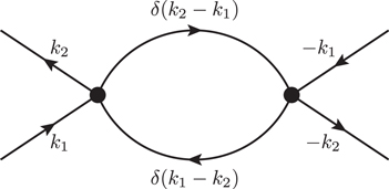
Figure 1. To maintain that the external momenta of the particle–hole diagram are pairwise antiparallel the diagram has to be restricted to forward scattering. This results in a strongly restricted phase space compared to figure 2. The contribution from this loop diagram is therefore negligible.
Download figure:
Standard image High-resolution image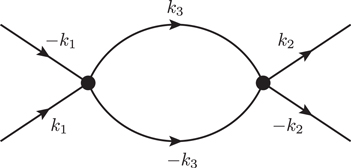
Figure 2. For the particle–particle channel the internal loops are equal with opposite momenta. The external momenta of the diagram are pairwise antiparallel.
Download figure:
Standard image High-resolution image2. Disorder-induced interactions
We assume that the introduction of disorder gives rise to two types of perturbations that might cause a transition out of the SC ground state. One of them breaks Cooper pairs to induce a transition towards an unpaired non-SC state. The other conserves pairs and either generates a transition into an unconventional SC state or into a non-SC paired state.
2.1. Pair-breaking perturbations
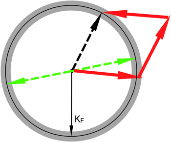
The simplest pair-breaking vertex consists of a single Cooper pair and an unpaired fermion or hole (1CP1e). The energy required to break the pair is provided by the unpaired particle, while momentum must also be conserved. For such a simple vertex we discuss the momentum conservation condition graphically (figure 3). The grey region represents the narrow band of slow modes around the Fermi momentum (KF). Modes outside the grey band are not important for the long-range behaviour and are integrated out. The incoming Cooper pair (dashed green) carries zero momentum and interacts with a single fermion or hole (dashed black) with a momentum within the grey region. The outgoing lines (red) have to conserve the incoming momentum and also lie within the narrow grey band. This restriction is only satisfied if two of the outgoing lines are antiparallel again. Therefore the only quantum process that survives the RG rescaling of the 1CP1e vertex describes conventional Cooper pairing in the presence of an unpaired fermion or hole.
Figure 3. Illustration of the momentum conservation condition for a three-particle interaction. Only momentum configurations within the grey region close to  survive the RG transformation. The momentum conservation for these slow modes forces two outgoing lines to remain antiparallel.
Download figure:
Standard image High-resolution image
The next higher-order pair-breaking vertex consists of a single Cooper pair and two unpaired fermions

with

Unlike the 1CP1e vertex, there are no kinematic restrictions for the 1CP2e vertex. When we perform the usual RG transformations and insert (12) into (15) we find that the 1CP2e vertex scales as s−3 at tree-level and hence is irrelevant with respect to the SC fixed point. The same is true for all higher-order pair-breaking vertices that consist of a single Cooper pair and two or more unpaired charge carriers. This resilience of BCS and high-temperature SC towards impurities has also been shown in other theoretical works [33, 34].
Apart from the tree-level term a relevant contribution may come from higher-order quantum corrections. However, as discussed in (appendix  can be neglected. However, for
  we cannot evaluate the Grassmann path integrals by induction anymore. In particular for
  higher-order quantum corrections will not vanish. For this regime of strongly disordered weakly coupled BCS-like superconductors, it is expected that during the SIT the SC ground state vanishes due to the breaking of Cooper pairs [1].
2.2. Pair-conserving perturbations
The disorder-induced direct localization of Cooper pairs during the SIT [21, 22] can be described as a pair-conserving interaction between paired fermions and impurities. In the limit of high disorder the free propagation of the fermion pair will be suppressed which eventually leads to localization. For a pair to survive an interaction with impurities, equal amounts of energy and momentum must be transfered for both fermions. This interaction can be described by the action

with  as the transferred energy and momentum respectively, and

To obtain the scaling of  with respect to the SC fixed point we perform the usual RG transformation. By inserting (12) into (17), the scaling of the
  vertex at tree level is

Hence, this pair-conserving Cooper pair-impurity interaction dominates at large length scales. This induces a transition away from the SC state towards a new fixed point. The ground state of this novel type of pairing interaction may either be an unconventional SC condensate or a non-SC gapped phase. To distinguish between the two scenarios it is sufficient to determine whether the ground state of the  fixed point is accompanied by the formation of a macroscopically coherent quantum phase (CQP).
2.2.1. Quantum phase coherence
It is known from the BCS theory that the condensation into the SC ground state is accompanied by the formation of a macroscopically CQP. The CQP condition is obtained by minimizing the energy expectation value  of the paired ground-state wave function

where  with respect to the quantum phase
  . The application of the Ritz variational method yields

for all  is a constant [35].
Since the BCS trial state (20) cannot describe systems containing unpaired charge carriers, which we must necessarily include to check the CQP condition subject to 1CP2e pair-conserving interactions, we chose instead of (20) the most general linear combination of states with paired and unpaired charge carriers

Here the amplitudes uK and vK( and
and  ) describe the occupation probability of unpaired fermionic (paired bosonic) states. Although we use a fermionic notation for clarity, the paired operators
  are effective boson creation operators. The application of an effective bosonic operator pair
  does not affect unpaired fermions. The notation
  indicates that configurations with multiple occurrence of the same index are not allowed i.e.
  and that each configuration appears only once. Equation (22) then describes product states of a single Cooper pair and its local environment consisting of two unpaired fermions.
For ordinary Cooper pair scattering this trial state has to reproduce the CQP. Indeed, when we apply the variational scheme on the energy expectation value the matrix element of the first half of the pair scattering reads

We note that only the paired states ( ) give a non-zero contribution. Since double occupancy is not allowed and each configuration must appear only once all terms where the states (
 ) are occupied can be pulled out of summation

Here  accounts for all remaining states that do not appear in the first bracket. When we apply
  only terms with an empty (
 ) state survive
For the expectation value we then find

where  denote the complex conjugates of
  . The notation
  implies that the initial trial state
  is reduced, i.e. the product state excludes the states
  . Minimizing
  with respect to the quantum phase reproduces the CQP condition (21).
Next we treat  as a competing interaction and check whether it disrupts the condensation of
  into a SC ground state. To minimize the energy expectation
  with respect to the quantum phases, the expectation value can be simplified as
with  . For the complex probability amplitudes of the unpaired holes we write as

and those for the Cooper pairs we write as

Here we can factor out the phase for all  to combine them to an overall constant phase. This is done by setting
  and substituting
  . To find the ground state the minimization has to be performed with respect to both, the phase as well as the amplitude. Variation with respect to the amplitude was performed in [36] for conventional BCS pairing. Here we are only interested in the phase coherence condition. Therefore we drop the amplitudes
  and keep the phase factors only to get

The Rayleigh–Ritz approach then yields
To simplify this expression we group δ-functions with the same sign and relabel the summations over S, T, W and P, Q, R according to

After further relabeling we combine the summations and set it equal to zero
The CQP condition is obtained if each individual summand in (28) becomes zero [35]. It is then easy to see that the CQP condition for conventional Cooper pairing (21) is one of infinite configurations to satisfy

Since the ground state is not exclusively realized for CQP condition but for an infinite number of non-CQP configurations, the ground state of the 1CP2e interaction is not SC.
3. Conclusion
In the first part of our work we present an extension of the well known RG method that allows us to determine the SC fixed point of a BCS-like Hamiltonian. From the comparison of pair-breaking and pair-conserving perturbations at the SC fixed point we find, that pair-breaking interactions are irrelevant on large length scales. While the SC state is resilient towards disorder induced pair-breaking [33], we identify a particular pair-conserving interaction (1CP2e) that describes the coupling of Cooper pairs in the presence of a disordered environment. For this unconventional pairing we find a relevant RG flow away from the conventional BCS ground state. In the ground state of this unconventional pairing, Cooper pairs are not coherent and therefore do not form a SC condensate. This behaviour is reminiscent of a PG-like state with pre-formed or disorder-modified Cooper pairs. We conclude that the observation of a second energy gap [13] may be related to the 1CP2e pairing. Moreover, because disorder-modified Cooper pairing is restricted to strongly disordered regions, we expect the formation of non-SC islands, separated by regions with a high SC order [29].
While the existence of pre-formed Cooper pairs can be anticipated, we are able to identify the 1CP2e mechanism as the actual quantum process that describes non-coherent Cooper pairs in a disordered BCS type system. Although we analyze a simplified Hamiltonian, the scalings of disorder induced pair-breaking and pair-conserving perturbations with respect to a s-wave fixed point, are universal. Therefore our results suggest that the formation of a PG-like phase is a general phenomenon of a disordered SC state instead of merely a peculiar property of HTSC materials.
Appendix A.: Effective action
The interaction part of the action S = S0 + SSC can be decomposed into

Here the first two terms, ![${S}_{\mathrm{SC}}[{\psi }_{\lt }]\;\mathrm{and}\;{S}_{\mathrm{SC}}[{\psi }_{\gt }]$](https://content.cld.iop.org/journals/1367-2630/17/10/103008/revision1/njp520348ieqn61.gif) consist of slow and fast modes respectively and
consist of slow and fast modes respectively and ![${\bar{S}}_{\mathrm{SC}}[{\psi }_{\lt },{\psi }_{\gt }]$](https://content.cld.iop.org/journals/1367-2630/17/10/103008/revision1/njp520348ieqn62.gif) contains fully mixed terms only. The quantum partition function separated into slow and fast parts is then of the form
contains fully mixed terms only. The quantum partition function separated into slow and fast parts is then of the form

We substitute the partition function  and take the average over fast fields to find
After averaging the full action (instead of  only) over the fast modes, we now obtain an effective action defined over the slow modes. For the RG operations the term
  only adds a constant factor which can be ignored. We therefore find for the modified effective action

Appendix B.: Grassmann path integration
The internal lines for quantum corrections are obtained by evaluating Grassmann path integrals of the form

where  is the action of the system and
  denotes the path integration over all possible
  configurations for the Grassmann numbers
  . For Grassmann numbers the integration simplifies according to


In particular, the Boltzmann weight in the path integral can be expanded as a Taylor series

where the action terms contain momentum and energy integrals themselves. We can discretize these integrals as

and

According to the Grassmann integration rules (36) the only non-vanishing terms in (37) must contain each field configuration exactly once. The implication of this is best understood by restricting the momentum and frequency phase space to a few allowed configurations. We demonstrate the evaluation of (34) for  allowed momentum values for a one-dimensional system first and then extrapolate to infinitely many allowed momenta. In this way we can understand how the RG transformation changes the path integral over fast modes. To begin, we consider only summation over the momenta (
 ) at symmetric locations around
  for a single frequency
  and find


when we measure the momentum with respect to  . In the multinomial expansion (37),
only the terms originating from  survive the Grassmann path integration. Using the anticommutation relations for Grassmann numbers the path integral (34) for two momenta and a single Matsubara frequency is

where  is suppressed in the argument.
Next we calculate (34) for the momenta ( ) with frequency
  .
.


where we again used  . From the multinomial expansion we obtain all relevant combinations that contain each Grassmann field exactly once
After rearranging the Grassmann fields the last three terms in (46) give a contribution of ![$2{U}^{2}[{\bar{\psi }}_{(1)}{\bar{\psi }}_{(-1)}{\psi }_{(1)}{\psi }_{(-1)}...]$](https://content.cld.iop.org/journals/1367-2630/17/10/103008/revision1/njp520348ieqn80.gif) . For the numerator we note that the term
. For the numerator we note that the term  reduces the multinomial expansion to
After Grassmann integration and regrouping of terms we find

The result for a single allowed momentum (43) is almost reproduced except for the additional  in the denominator. The trend of a growing denominator with respect to the numerator continues for the case (
 ) with frequency
  where we find

The additional terms that prevent cancellation as in (43) are

Because of the restriction  the Matsubara frequency
  is the leading term in
  and since
  the leading additional terms in (50) have the same sign. When we compare (48) and (49) with (43) we conclude that in the limit
  the number of additional terms that prevent cancellation increase, i.e.
  and thus
  .
.
In summary, the convergence of fractions of Grassmann path integrals remains trivial only at the fixed point where the multinomials in the numerator and denominator contain the same potential  . Moreover, it is interesting to note that for
  the additional terms in
  come with alternating signs and therefore the average
  and hence quantum corrections do not vanish. This indicates that the definition of a fixed point with a repulsive interaction (
 ) is ambiguous. We also note that for general perturbations (
 ) of the SC state the calculation of averages of the form
  is not trivial and a simple comparison of the number of terms in the numerator and denominator in general is not feasible.