


Abstract
Here, we enhance the capabilities of the atomic force microscope (AFM) to show that force profiles can be reconstructed without restriction by monitoring the wave profile of the cantilever during a single oscillation cycle. Two approaches are provided to reconstruct the force profile in both the steady and transient states in what we call single-cycle measurements. The robustness of the formalism is tested numerically to recover complex but relevant interactions. With single-cycle measurements, we add high temporal resolution (possibly microsecond range) to the spatial resolution of AFM. The access to simultaneous high throughput and high sensitivity further opens the door to a variety of feedback options for imaging.
Export citation and abstract BibTeX RIS

Content from this work may be used under the terms of the Creative Commons Attribution 3.0 licence. Any further distribution of this work must maintain attribution to the author(s) and the title of the work, journal citation and DOI.
1. Introduction
Atomic and nanoscale interactions that govern the macroscopic behavior of materials [1] originate from a length scale that can be accessed using the atomic force microscope (AFM) [2]. Since its advent and due its high spatial resolution, AFM has enabled probing single nanostructures [3], mapping heterogeneous compositional variation in surface properties [4–8], studying molecular interactions [9, 10] and larger biological systems [11] and even identifying single atoms in surface alloys [12] and discriminating bond order [13]. In principle, the versatility of the instrument arises from the fact that single atoms and nanostructures can be probed with a nanoscopic tip and with high precision by monitoring and controlling the structure onto which the tip is mounted: typically a micro-cantilever. When the cantilever is vibrated, the rich dynamics arising from the nonlinear forces has led to the branching of AFM into several modes of operation [14–17]. Nevertheless, a general trend in the community can be identified in the attempt to extend its capabilities toward extracting more quantitative information and increasing sensitivity [18–20] and throughput [11, 21]. The interest in extracting quantitative information about interaction forces is clearly related to identifying and decoupling chemical, mechanical and other properties that are characteristic of the material. In short, accurately measuring nanoscale forces should enable evaluating and discerning interactions such as the activation of atomic processes [9, 22], atomic bonding [23, 24], materials elasticity of even small and soft biostructures [25] and the mechanisms involved in complex thermodynamic processes [26]. Here, we focus on force reconstruction where no restriction is placed in terms of the nature of conservative or dissipative forces, or even on whether the fundamental period of oscillation coincides with the period of the driving force as can happen experimentally [27, 28]. Two methods are proposed. The first method, which we term the modal analysis method, is developed for cantilevers oscillating in the steady state taking into account the base excitation. The formalism is tested numerically by implementing complex hysteretic interactions where other standard force reconstruction methods fail. We term the second method the single-cycle method. The single-cycle method is based on monitoring the waveprofile of the cantilever with a finite number of points along its axis. We show that, in this way, variations in force can be accurately probed, in principle, with submicrosecond resolution. Although both methods lead to rapid and sensitive force reconstruction, there are technical challenges involving implementation that we also discuss.
2. Force reconstruction schemes: assumptions and challenges
In their simplest form, force measurements are performed in dc modes by monitoring the cantilever static deflection as a function of tip–sample separation [29]. In general, however, dc operation suffers from the downside of the 1/f noise factor [30, 31], which is particularly critical when using relatively soft cantilevers, and lacks the capacity to obtain compositional contrast related to dissipative mechanisms [8, 31, 32]. Moreover, the dc mode of operation further fails to provide compositional contrast due to conservative interactions while imaging [16] and also in the interpretation of hysteretic dissipation in the long range [29, 33]. Dynamic AFM overcomes the above limitations in the sense that the energy stored in the cantilever competes with conservative and dissipative tip–sample interactions in the control of cantilever dynamics [31, 34]. Furthermore, in the dynamic modes, the cantilever-stored energy transferred to the tip–sample junction provides an added channel of compositional contrast and allows probing dissipation even in the non-contact region [8, 32, 35]. Dynamic AFM, however, comes with the cost of added complexity in the analysis of the motion and in the electronics required for operation [31].
The integral form of the equation of motion valid for all oscillation amplitudes in single-mode dynamic AFM was inverted by Sader and Jarvis in 2004 [36]. More recently, Katan et al [30] proposed employing the Sader–Jarvis solution to reconstruct the force in amplitude modulation (AM)-AFM. The Sader–Jarvis–Katan expression has proved to be very powerful and robust, and it is a testament to the robustness and accuracy of atomic force reconstruction in dynamic AFM modes [37, 38]. Other methods where similar assumptions are adopted in the derivation have been proposed by Hölscher [39], Lee et al [40] and Hu and Raman [41]. These methods rely on the minimum distance of approach dmin and could thus be termed as minimum distance of approach methods. In general, such formalisms can be employed to reconstruct the conservative component of the force as well as a generalized damping coefficient. Deviations in force might be expected, however, when the tip is vibrating in a highly damped medium, or more generally, when higher harmonics are excited [42]. Other cases where the formalism fails are physically relevant and are discussed below. Alternatively, the excitation of higher harmonics can be acknowledged by employing the differential form of the equation. The interesting physical implication is that all the details about the instantaneous nonlinearities of the tip–sample force Fts can be recovered [43]. Although the theoretical work in [43] showed the power of the differential form to recover details of complex interactions, it neglected higher modes. Stark and Heckl [44], however, already formulated the problem of cantilever vibration using modal analysis over a decade ago. Some have recently pursued the ideas of Stark and Heckl for force reconstruction [45], but the difficulties related to higher harmonic detection have also led to torsional modes of operation where standard micro-cantilevers are slightly modified [21]. More recently, the simultaneous excitation of higher modes is being employed to provide quantification without compromising throughput [7, 18, 19, 46].
It could be argued that methods relying on the dmin concept are the most extensively used since they typically require the use of standard equipment only. On the other hand, hysteretic forces might be completely missed by these methods [47]. Let us, for example, consider surface energy hysteresis. This is a key dissipative mechanism that is assumed to control nanoscale energy dissipation. Theoretical as well as experimental investigations have been conducted for years from the classical [48] and atomistic perspectives [49], or combinations of both [9, 50, 51]. From an interaction point of view, hysteretic dissipation entails that the magnitude of the force while the tip is approaching the surface is lower than its magnitude while the tip retracts. A simple model that does not take into account possible variations in surface energy γ as a function of distance can be written for a short-range hysteretic force Fi:

where i ≡ a during tip approach and i ≡ r during tip retraction, and where γ is the surface energy (γa < γr implies energy dissipation) and R is the tip radius. Hysteretic forces that activate and terminate at specific tip–sample separations have also been considered for over a decade by several groups [52–55]. Here we refer to such hysteretic behavior as a don–doff mechanism. A physically relevant and important case where these hysteretic forces are believed to prevail is in the presence of capillary neck formation and rupture [54, 56]. Other relevant scenarios might involve bond formation and rupture due to chemical affinity, or other, between the tip and the sample [57, 58]. A simple mathematical formulation of Fon–off forces is
In this formalism, κ acts as a memory parameter that starts with κ = 0, d is the tip–surface separation measured from the sample surface and doff > don. If the tip crosses don, where d < don, κ = 1. If the tip retracts past doff, where d > doff, κ = 0. The physics of the force in equation (2) is different from that in equation (1), in that the Fon–off force only dissipates energy in a cycle if the tip passes through both don and doff. An example of the predictions by the Sader–Jarvis–Katan method when hysteretic forces, such as those in equations (1) and (2), are considered together with standard [59], conservative attractive [60] and repulsive [61] forces is shown in figure 1. The protocol and implementation of these forces for numerical integration have been recently discussed in light of the Sader–Jarvis–Katan solution [62] and a similar protocol has been followed here (see supplementary material, available from stacks.iop.org/NJP/15/083034/mmedia). A discussion of the predictions follows.
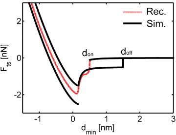
Figure 1. Tip–sample interaction profile where conservative forces are present simultaneously with short-range surface energy hysteresis and long-range hysteresis (don–doff). Fts (Sim.) stands for the true force profile used in simulations for the conservative forces and Fts (Rec.) is the recovered conservative force according to the Sader–Jarvis–Katan formalism. Simulation parameters: spring constant k = 40 N m−1, resonance frequency f0 = 300 kHz, quality factor Q = 450, free amplitude A0 ≈ 25 nm, Young's modulus of the tip Et = 120 GPa, Young's modulus of the sample Es = 1 GPa, tip radius R = 8 nm, surface energy γa = 10 mJ m−2 and γr = 20 mJ m−2.
Download figure:
Standard image High-resolution imageIn figure 1 the reconstructed force (dashed red lines) follows very accurately (errors of less than 5%) the conservative long-range force (black lines) prior to d = don. The metastability of the don–doff region modeled by equation (2), however, is not recovered and only the approach path can be extracted. Note the discontinuity and overshot in Fts observed at d = don resulting as a consequence of the onset of equation (2). It is clear from the figure that information regarding the retraction path in this metastable region is lost. During mechanical contact, i.e. d < a0, the hysteretic force from equation (1) comes into action. Here the force recovered with the Sader–Jarvis–Katan formalism lies in between the approach and retraction paths. The accuracy of the force values deteriorates (not shown) as the tip further indents into the surface [36]. This is due to the effects of higher harmonics, the larger mean deflection relative to oscillation amplitude and the increase in frequency shift [63]. Errors in the recovered Fts values in the region of mechanical contact might lead to inaccuracies in the calculation of important nanoscale sample mechanical properties, such as peak forces [18] and elastic modulus [25].
A highly sophisticated instrument such as the AFM should be able to provide information about relevant nanoscale interactions, such as those related to the above mechanisms in equations (1) and (2), with no restrictions on the nature of the interaction. In what follows, two methods are presented that overcome the limitations of force reconstruction methods based on the minimum distance of approach, i.e. dmin, and, in general, the recovery of effective force and damping parameters.
3. Force reconstruction in steady-state oscillation: the method of modal analysis
The one-dimensional Euler–Bernoulli beam equation that governs the dynamics of a rectangular beam can be written as follows [64]:

In this equation, the elastic modulus E(x) and moment inertia I(x) are assumed to be constant along the length of the cantilever L, where x is the coordinate along the cantilever axis. The damping in the system is accounted for by a0 and a1 [44]. The mass per unit length μ(x) is also considered constant along the cantilever length. The force tip–sample fts is localized at the end of the cantilever.
The boundary conditions that govern the cantilever motion are
Here, u(x, t) is referred to an inertial reference frame. If the equation is projected onto a non-inertial reference frame by expressing the cantilever deflection w(x, t) as

where y(t) is the base motion [64], the inertial terms appear naturally in the equation as an equivalent excitation force and all the boundary conditions are null. Then
Expansion of w(x,t) as a series of eigenmodes (see appendix A) produces

where ϕm(x) is the normalized eigenfunction of the mth mode. We further write ϕ(L) = 1, and consequently the measured tip deflection is zm(t). Substituting equation (6) into (5), multiplying by ϕm(x) and integrating over the length of the cantilever L results in (see appendix A):
Or more compactly (see appendix A)

where equation (8) is written in terms of generalized modal quantities: generalized modal mass Mm and generalized modal quality factor Qm. The effect of base excitation (quantity in square brackets) is translated into an equivalent excitation force.
Furthermore, in the frequency domain, the steady-state dynamics follows from equation (8):

where Ω is the angular frequency of the base excitation. Or, in a more compact form

where the constraint

is employed and where Adn and θn are the amplitude and phase of the nth harmonic of the base excitation. The quantity Hmn is used in equation (10) to replace the quantity in brackets in equation (9).
We demonstrate the analysis for a three-mode system with no loss of generality where equation (10) can be written as
Multiplying by the inverse of the MH matrix, we obtain
The generalized expression for the tip–sample force for the nth harmonic Fn ejγn follows at once from equations (11) and (13) and can be written as
Finally, the instantaneous net tip–sample force can be written as

It is worth noting that it is a common practice to drive the base at a single frequency Ω. In this case Adn = 0 for all but n = 1.
The validity of equation (14) is next tested employing numerical results obtained from finite element (FE) simulations. In the FE simulations, the cantilever oscillates via base excitation and the tip–sample force includes both types of hysteresis discussed with the use of figure 1, i.e. equations (1) and (2). Figure 2(a) shows five oscillations of the steady-state cantilever deflection as a function of time. A Fourier transform reveals the frequency content (figure 2(b)). From the amplitude spectrum, one can deduce the number of harmonics that could be detected from an experimental point of view. In particular, in figure 2 harmonics contribute with amplitudes in the pm range or more up to the fifth eigenmode.
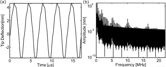
Figure 2. Tip deflection waveform analysis. (a) Five cycles of the steady-state tip deflection w(L, t) of the cantilever as a function of time. Clear wave distortion can be observed indicating the presence of higher harmonics. (b) Amplitude spectrum of the deflection waveform showing equally spaced amplitudes of the higher harmonics. The plot can point out the significant number of modes that can describe the cantilever motion. Simulation parameters: L = 160 μm, A = 25 × 5 μm2, ρ = 2300 kg m−3, Et = 200 GPa and Q1 = 9.
Download figure:
Standard image High-resolution imageEquation (14) has been applied to the system discussed in figure 2 to recover the force component for each harmonic and fts(t) has been reconstructed with the use of equation (15) as shown in figure 3(a). In this example, 60 harmonics have been employed with a fast Fourier transform (FFT) resolution of about 30 Hz. Resolution limitations are due to computational cost in the FE method and also to numerical noise. Resolution limitations, however, should not affect experiments. In the force plot in figure 3(b), the reference value for the tip position u(L, t) is arbitrary since, as in the experimental case, the location of the sample surface is unknown.
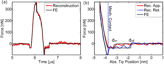
Figure 3. Force reconstruction in the steady state using the method of modal analysis. (a) Force waveform as a function of time. The reconstructed force using equation (14) agrees very well with the force employed in FE. (b) Approach and retract reconstructed force curve as a function of the absolute tip position u(L, t). The short-range hysteretic region is very well captured. The approach curve demonstrates the constant force value before mechanical contact. The don–doff discontinuities are not very well reproduced, but clear splitting between the forces is observed and the extension of the region is also accurately described. Simulated force parameters: don = 0.5 nm, doff = 2 nm, H = 3 × 10–19 J, R = 10 nm, γa = 10 mJ m−2, γr = 40 mJ m−2, Es = 60 GPa and Ad = 2 nm.
Download figure:
Standard image High-resolution imageIn summary, multimodal analysis as described in equations (3)–(15) is shown to lead to the recovery of the approach (red lines) and retraction (blue lines) paths (figure 3(b)) employed in the FE simulation (black lines) as a function of the tip position. In particular, metastability in the recovered force is observed at distances don ⩽ d ⩽ doff. The oscillatory behavior of the recovered force signal in both the approach and the retraction paths is a consequence of the superposition of harmonic waves and discontinuities lead to the Gibbs phenomenon [43, 65] as expected. It is clear that the presented modal analysis is powerful and allows capturing the details related to discontinuous and arbitrarily complex interactions. Nevertheless, the approach fails to capture dynamic phenomena that have a time scale shorter than the time needed by the cantilever to reach steady state, i.e. milliseconds [43, 52]. On the other hand, equation (15) and the distortion of the waveform in figure 2(a) imply that a single cycle already contains all the information related to the instantaneous tip–sample force. It should then be expected that a suitable formalism would allow carrying out single-cycle force reconstruction leading to temporal resolution at least three orders of magnitude larger, i.e. microsecond. Such formalism is discussed next.
4. Force reconstruction in transient state oscillation: differential quadrature method (DQM)
In the method of modal analysis, the force is localized at the end of the cantilever with a delta function as in equation (3). On the other hand, the boundary conditions are those of a free vibrating cantilever. Hence, the mode shapes are easily evaluated and employed to reconstruct the force. In reality, however, the tip–sample force that is being probed is acting in the normal direction. This means that there is a shear force acting at the cantilever's end (see boundary conditions in equation (17)). Thus, one should be able to estimate the instantaneous force acting on the cantilever from the third (spatial) derivative of the cantilever deflection. This idea, however, is immediately challenged mathematically as well as practically by the fact that the closed-form expression that describes the instantaneous cantilever deflection is missing. Besides, it is noted that the force has a dependence on the tip–sample separation.
In order to surmount these obstacles, here, the differential quadrature method (DQM) [66] is employed. DQM is a numerical approach that can evaluate such derivatives fairly accurately with a considerably small number of sampling points along the cantilever axis [67–72]. In short, in DQM the derivative of a function with respect to a variable at a given point is approximated as a weighted linear sum of the function values at all discrete points in the range of that variable [67]. In terms of dimensionless variables, the rth-order derivative of a function w(ζ) at ζ = ζi, defined between 0 and 1 with N discrete grid points, is given by

The elements of A(r)ij are the weighting matrix coefficients corresponding to the rth-order derivative. The details of calculating A(r)ij are provided in appendix B. We next utilize a simpler form of equation (3) where the stiffness proportional damping coefficient is neglected. The expression reads

where
Then, a dimensionless variable ζ = x/L is introduced in order to rewrite the partial differential equation, i.e. the governing equation of motion of the cantilever, as
From DQM standard theory, the following set of equations directly follows:

Note that equation (19) with the corresponding boundary conditions has been recently employed [73] to simulate and interpret the dynamics of an oscillating cantilever in the presence of conservative long-range van der Waals attractions [60] and conservative short-range forces. The short-range forces were modeled with the DMT model of contact mechanics [61], which is common practice in AM-AFM [31]. The study in [73] gives an insight in terms of how the resonant frequencies, as well as the mode shapes, of the cantilever behave as a function of tip–sample separation. In fact, the formalism allows incorporating the boundary conditions into equation (19) to reduce the number of coupled equations to be solved [74]. The system of equations is then equivalent to

where
and where
It should be recalled that the aim here is to force reconstruction in a single oscillation cycle. For this purpose, we focus our attention on equation (21). Note that equation (21) establishes that despite the relative complexity of the theoretical foundation of DQM, the force reconstruction is trivial. The procedure can be described as follows. (i) The deflection of the cantilever in the time domain is recorded, simultaneously, at specific locations on the cantilever according to the grid defined in appendix B and for any period of time. (ii) The deflections at each point are added up, after being scaled by a weighting coefficient Cj. (iii) Finally, the instantaneous tip–sample force fts(t) is this summation multiplied by EI/L3 as in equation (21).
It is worth noting that no assumptions related to cantilever motion are made in this approach except that the governing equation of motion is described by the Euler–Bernoulli equation (small deflection assumption). That is, no assumptions are made in relation to the state of the dynamics of the cantilever. Thus, the formalism in equation (21) works equally well in the steady state and in the transient state of vibration, i.e. it allows real single-cycle analysis.
FE is employed next to demonstrate the use of equation (21) as before. In this case, however, the cantilever deflection is recorded at specific points along its axis as defined by grid spacing (see appendix B). Note that an eight-point grid is sufficient to extract accurate results. Also note that the summation in equation (21) starts from four after including the boundary conditions. Thus, the deflection has to be recorded at five different locations along the cantilever axis only as shown in figure 4(a). The force in time, as reconstructed by the DQM method (red lines), is shown in figure 4(b) where it is observed that it follows the tip–sample force employed in the FE simulations (black lines). The force is further plotted in terms of the absolute tip position in figure 4(c). The reconstruction captures all the features of the force curve including the abrupt drop in force at the don–doff distances. It is also interesting to note that these force plots have been generated in the transient state of vibration (see figure 4(a)).
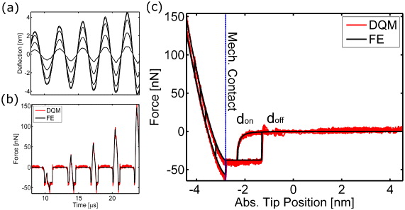
Figure 4. Force reconstruction using DQM. (a) The tip deflection waveform recorded at five grid points along the cantilever axis as a function of time. The higher the deflection is, the closer the point to the cantilever end. Clear wave distortion is observed when the grid point is closer to the cantilever base. (b) Verification of the DQM force reconstruction waveform using FE. (c) Force field as a function of the absolute tip position with excellent reconstruction of the force field in short as well as long-range hysteretic regions even at points of discontinuities. Simulated force parameters: Don = 0.5 nm, Doff = 1.5 nm, H = 3 × 10–19 J, R = 20 nm, γa = 10 mJ m−2, γr = 40 mJ m−2, Es = 10 GPa, Q1 = 500 and Ad = 200 pm.
Download figure:
Standard image High-resolution imageAn FE simulation has been next conducted where a dynamic tip–sample force has been employed. That is, the expression for the tip–sample force has been varied during the simulation. This situation could be analogous to physically relevant cases where the forces vary with time at a given sample location. For example, this situation could exemplify the case where a tip interacts with water layers on a sample's surface and where the volume of water increases with time due to the proximity of the tip. Similar processes might be present due to the segregation of matter on the surface as thermodynamic equilibrium is reached [75]. Other examples might include the creeping of the tip and/or sample, plastic deformation [76], the motion of ions on the surface as the tip taps on a given location [77] or charge transfer [78]. The reconstruction of time-varying forces is discussed next with the use of figure 5.
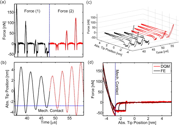
Figure 5. Transient force field reconstruction. Reconstructed (a) force and (b) tip position as a function of time in a transient state. In the simulation, two forces are included and incorporated dynamically as the tip vibrates. Force (1) is shown with the use of black lines and includes short- and long-range hysteretic forces. Force (2) is shown with the use of red lines and only includes conservative forces. The DQM method captures the immediate transition from force (1) to force (2) confirming that forces that vary in time can be reconstructed even as the cantilever oscillates in the transient state. (c) 3D force plot as a function of absolute tip position and time showing the transition from force (1) to force (2) as the cantilever oscillates in the transient state. (d) Projection of the two force profiles against the absolute tip position. The two distinct forces are reconstructed.
Download figure:
Standard image High-resolution image
In figure 5, as the cantilever oscillates, two force profiles have been probed. The first force profile, force (1) (black lines in figures 5(a)–(c)), includes the two hysteretic force components in (1) and (2). The second force profile, force (2) (red lines in figures 5(a)–(c)), includes only conservative forces (see supplementary material, available from stacks.iop.org/NJP/15/083034/mmedia). In the FE simulation, force (1) was dynamically exchanged for force (2) as the cantilever vibrated, i.e. approximately after the third period of oscillation shown in the figure. Note the change in color there. Both experimentally and in the simulations, this instantaneous transition in force induces transient cantilever vibrations, but equation (21) can handle these situations as shown in figures 5(c) and (d). Figure 5(c) shows a three-dimensional (3D) plot of the tip–sample force as a function of time and tip position. The transition between force profiles is distinctively observed in the figure at approximately the center of the plot, i.e. time ≈47 μs. The force reconstruction for both force profiles as a function of tip position is shown in figure 5(d).
The discussion in this work has mainly focused on the formulation and the validation of force reconstruction techniques that can probe material properties, chemical reactivity and other complex phenomena even in the transient state of cantilever vibration. Nevertheless, an important aspect also to be addressed is the applicability of this work from an experimental point of view. As stated, the accuracy of the modal analysis depends on acquiring an FFT with sufficient resolution. Insufficient bandwidth of the measurements will result in the loss of higher harmonics, causing severe limitations on the force reconstruction scheme. This issue has a general relevance and even extends to T-shaped cantilevers and torsional modes [79, 80]. Improving the detection of higher harmonics might be technologically challenging but not unachievable and should steadily improve together with improving feedback systems and, in general, electronic support. In particular, the implementation of the steady state or modal analysis should be achieved with current AFM setups. For example, with the standard optical lever method [81], the waveform for a tip oscillating at a constant separation from the surface can be recorded for any duration. It is noted, however, that the modal shape detection with the optical lever method is very sensitive to the position of the laser spot along the cantilever. Moreover, the calibration of modal shapes is challenging and might significantly deviate from that deduced from ideal rectangular cantilevers. Nevertheless, future experiments and theory should dictate which the optimum cantilever and oscillation detection schemes are. Technological challenges involving phenomena such as thermal drift and other specific challenges, for example whether there is an optimum set of operational parameters, are also problems that should be considered in future applications. Other important issues relate to the calibration of the InvOLS [82] and modal generalized quantities such as Mm and Qm along with the resonance frequencies ωm. Accurate calibration of these parameters is key in obtaining meaningful results [7, 35, 83].
From a theoretical point of view, and due to its relative simplicity, the DQM method can also be employed for steady-state analysis. From a practical point of view, the DQM method is expected to yield satisfactory results when applied to rectangular cantilevers whose dynamics can be approximated with the Euler Bernoulli's equation. Stringent control on cantilever non-idealities will guarantee the validity of the approach in the present formalism. Future developments with the use of standard cantilevers should take into account the actual cantilever geometry and this should lead to technical modifications in the formalism. Moreover, the implementation of the DQM method is not straightforward with conventional AFM setups. In principle, a multi-laser system is required to simultaneously monitor the cantilever shape at very specific locations during its interaction with the sample. Such technological issues, however, are being currently actively dealt with by both research groups and manufacturers [84]. For example, the spatial shape of the cantilever has been mapped during tip–sample interaction. With optical techniques, Kiracofe and Raman [85] employed a Doppler vibrometer to decouple base and cantilever motions. Reinstaedtler et al [86] utilized an optical Michelson heterodyne interferometer to scan the cantilever surface. Furthermore, even with a commercial device such as the Cypher AFM from Asylum research, the feedback loop can be disabled and the laser spot can scan automatically along the cantilever axis to provide a continuous waveform for the cantilever motion. Such experimental efforts, however, are typically employed by specialized groups and are still not common in the AFM community. Furthermore, employing these techniques is not trivial and poor detection of the motion of the cantilever and inconveniences caused by thermal noise might still be significant even with the use of such sophisticated detection techniques. Cantilever non-idealities along with the base noise of the system further complicate the analysis. Nevertheless, they provide evidence that the DQM approach might be leveraged with minor changes in AFM setups and, in any case, the interest in the field suggests that in the near future standard AFMs might ship with the required hardware and software to conduct the experiments.
5. Conclusion
Two methodologies have been presented and developed here that have the potential to deal simultaneously with high sensitivity and high throughput scanning and with nanoscale resolution. The two techniques have been termed (i) the modal analysis and (ii) the DQM method. Both methods lead to instantaneous tip–sample force reconstruction without imposing restrictions on either the physical origin or profile of surface forces. Since the force profile encodes all the required information about physical, mechanical and chemical properties of samples, the information provided by these techniques enables access to such nanoscale phenomena and its quantification. Importantly, the present methodologies have been shown to overcome (i) the limitations of current and standard force reconstruction techniques where effective forces and damping parameters are employed, (ii) the limitations of current and standard force reconstruction techniques where hysteretic forces cannot be accurately reconstructed and (iii) the limitations in speed or throughput posed by force reconstruction techniques that require probing the whole cantilever–sample separation.
The limitations in terms of the practical implementation of the proposed techniques have also been discussed in detail, since it is clear that accurate detection of the full motion of the cantilever is crucial and non-trivial in the force-reconstruction methods here. It should be stated, however, that while accurately monitoring the deflection of the cantilever in detail remains experimentally challenging, theoretical developments, more accurate electronic and control equipment and careful experimentation should tell what the limits of detection are. It is thus expected that future advances should only increase the accuracy of the proposed methods and these, in turn, will support the development of nanoscale characterization.
Appendix A.: Steady-state force reconstruction: modal analysis
The solution procedure for the equation of motion of a freely vibrating cantilever is commonly addressed in structural dynamics textbooks [87]. Hence, the relevant equations to the method of force extraction in the steady state are only reviewed in this appendix.
The modal analysis of an un-damped free vibration equation requires solving an eigenvalue problem. For a free vibrating cantilever, the eigenvalues of the problem can be determined from the characteristic equation

where ωm is the angular resonance frequency of the mth mode.
The equation has infinite number of solutions, where the first three numerical values are λ1L = 1.875, λ2L = 4.694 and λ3L = 7.854. The eigenvectors (mode shapes) ϕm(x) must satisfy the boundary conditions for a freely vibrating cantilever [ ] and have the following expression:

The eigenvectors are orthogonal and normalized, meaning that

where δmn is the Kronecker delta (δmn = 1 if m = n, otherwise δmn = 0). The eigenfunctions are further utilized to describe the cantilever motion as a coordinate system as seen in equation (6). When substituted back in equation (5), we employ condition (A.3) to reach the following expression:
It is noted that
The integrals (A.4) take definite values, so the formalism is simplified to the expression seen in equation (7). To proceed, it is noted that the problem is transformed to uncoupled set of equations that resemble harmonic oscillator motion with generalized modal parameters. The coefficients of the cantilever acceleration are termed as generalized mass Mm = μαm, while those of the cantilever displacement are termed as generalized stiffness Km = EIαmλm4. Accordingly, we reach the same relationship of the mass and stiffness of a harmonic oscillator

Finally, a generalized damping term Λ is proposed where

However, it is common for harmonic oscillator analysis to report the damping in terms of the quality factor Q. So the generalized damping can be put in standard form as follows:

With the aid of generalized terms, equation (8) directly follows.
Appendix B.: Transient state force reconstruction: DQM
In the DQM, the weighting coefficients A(n)ij of the nth-order derivative can be determined through the recurrence formulae as follows. The off-diagonal elements of the weighting coefficient matrix of the first-order derivative are
Then, the off-diagonal elements of the weighting coefficient matrix of higher-order derivatives are estimated by

The diagonal elements of the weighting coefficient matrix are then determined through
Finally, the shifted Chebyshev–Gauss–Lobatto points are adopted as the basic mesh points with a stretching coefficient ε = 0.4 [88], so

