


Abstract
We discuss the transport properties of a single photon in a one-dimensional waveguide with an embedded three-level atom and utilize both stationary plane-wave solutions and time-dependent transport calculations to investigate the interaction of a photon with driven and undriven V- and Λ-systems. Specifically, for the case of an undriven V-system, we analyze the phenomenon of long-time occupation of the upper atomic levels in conjunction with almost dark states. For the undriven Λ-system, we find non-stationary dark states and we explain how the photon's transmittance can be controlled by an initial phase difference between the energetically lower-lying atomic states. With regard to the driven three-level systems, we discuss electromagnetically induced transparency in terms of the pulse propagation of a single photon through a Λ-type atom. In addition, we demonstrate how a driven V-type atom can be utilized to control the momentum distribution of the scattered photon.
Export citation and abstract BibTeX RIS

Content from this work may be used under the terms of the Creative Commons Attribution 3.0 licence. Any further distribution of this work must maintain attribution to the author(s) and the title of the work, journal citation and DOI.
1. Introduction
Much of the recent progress in quantum photonics as well as in circuit and cavity quantum electrodynamics is based on considerable advances in micro- and nanofabrication techniques and on improvements in the understanding of the underlying physical mechanisms. Different approaches exist for the realization of quantum optical circuits, e.g. via superconducting devices [1, 2], semiconductor structures [3] or hybrid systems [4]. For instance, recent works have demonstrated the efficient coupling of quantum dots as single photon sources to the modes of integrated waveguiding elements [5] as well as the generation and manipulation of arbitrary one- and two-photon states in such systems [6].
Although the above approaches differ widely in materials and operating wavelenghts, their basic building blocks exhibit the same characteristics: they consist of low-dimensional waveguiding structures with embedded quantum impurities so that quantum interference can be utilized efficiently. From a theoretical vantage point, already the investigation of the apparently simple model of a single two-level system (2LS) embedded in a one-dimensional (1D) waveguide leads to interesting effects such as an energy-dependent mirror [7–10] or strong nonlinearities on the few-photon level [11–17]. In addition, it has recently been proposed to utilize these systems as local quantum probes within a Hong–Ou–Mandel setting [18].
These systems exhibit an even richer behavior (and associated level of complexity) if the 2LS is replaced by a three-level system (3LS). Already stand-alone 3LSs display interesting physical effects such as electromagnetically induced transparency (EIT) [19] and the possibility of adiabatic population transfer [20] that simply do not occur in 2LSs. EIT with classical radiation in the case of a single emitter embedded in a 1D system has been realized with the help of superconducting devices [21, 22]. Furthermore, 3LSs give the possibility to control and tune effects that do occur in 2LSs, but only in very specific situations that might be difficult to realize and/or maintain experimentally—the perfect mirror effect alluded to above being a case in point [23–25].
The stationary scattering properties of single- and two-photon plane-wave states in 1D waveguides with linearized dispersion relations and embedded driven and undriven 3LS have been analyzed recently [26–29]. Specifically, EIT for single photons and single atoms has been described [27, 28], a proposal for a single-photon transistor has been formulated [27], and 3LS-mediated photon-bunching effects [28, 29] similar to the 2LS case [7, 8] have been found.
In this work, we give a detailed analysis of the scattering properties and dynamics of single-photon pulses that propagate in 1D waveguides with arbitrary (i.e. nonlinear) dispersion relations and interact with a single driven or undriven embedded 3LS. Specifically, we carry out analytical calculations for single-photon plane-wave states in the stationary regime and perform time-dependent simulations for single-photon pulses. The paper is organized as follows. We start with a description of the fundamentals in section 2. This is followed by sections 3 and 4, where we present the results of our work on undriven and driven V- and Λ-3LS, respectively. Specifically, we will see how a long-time occupation of upper atomic states can be reached, we consider the role of dark states in the undriven systems and how the relative phase of the atomic states can influence the single-photon scattering properties. In all these cases, we focus on the differences between the results of stationary plane-wave calculations and dynamical pulse–state simulations. In addition, we examine effects that result from the, in general, nonlinear dispersion relation of the waveguiding system. In section 5, we summarize our work and provide a brief outlook.
2. Fundamentals
We start by introducing the Hamiltonian of the above-described class of systems. Similar to other works [7–15, 27, 28], the Hamiltonian  consists of three parts:

Here,  represents a 1D waveguide for which we assume a tight-binding model that describes the quantized modes of the waveguide on an equidistant real-space lattice (lattice spacing a = 1) with nearest neighbor coupling J (ℏ = 1):

The operators  and
and  denote the bosonic creation and annihilation operators for photons at site x of the waveguide. The first term of Hamiltonian (2) represents the photonic on-site energy ω0, i.e. the eigenenergy of an uncoupled site. The second term describes the hopping between neighboring sites with strength J. Such a model features one band with a cosine-shaped dispersion relation
  k = ω0 − 2J cos(k) that is generic in the sense that it exhibits approximately linear dispersion near the center of the band and features band edges (cut-off frequencies) where the dispersion relation is approximately quadratic and a slow-light regime is formed. Both features are characteristic of a number of physical systems such as mono-mode fibers, ridge waveguides and coupled-resonator as well as photonic crystal waveguides. The latter two systems correspond particularly well to a tight-binding model. Clearly, systems with more than one band and different dispersion relations can be modeled by going beyond the nearest-neighbor interaction. For instance, in the case of photonic crystals this is facilitated by a Wannier function approach [30]. Such models allow for the quantitative descriptions of realistic systems via the same numerical methods that we use below, but such models considerably complicate the analytical treatment without changing the qualitative features. At this point, we would like to note that several of the works mentioned above [7, 8, 11–13, 27, 28] utilize linearized dispersion relations, which are extended to infinity, i.e. the physics associated with slow-light regimes, band edges and band gaps has not been discussed in these works.
States of natural atoms have well-defined parities, and radiative dipole transitions are only allowed between states of different parity. Therefore, exactly one of the three transitions of a 3LS is dipole-forbidden. Consequently, one distinguishes between three configurations, the so-called V-, Λ- and ladder configurations. In the V-configuration, a single ground-state dipole couples to two excited states, which themselves do not couple (see figure 1). Conversely, in the Λ-configuration, two energetically lower lying states dipole couple to one common excited state (see figure 4). In the ladder-configuration, a ground-state dipole couples to an energetically intermediate state that in turn dipole couples to an energetically higher-lying state. The corresponding Hamiltonians  will be specified in the respective subsections that deal with driven and undriven 3LS. In the context of single-photon transport the ladder-configuration is considerably less important, since in the undriven case and in the single excitation regime (see below, equation (4)) the highest level is irrelevant and the physics is the same as for a 2LS consisting of the two lower states of the ladder system. The driven cases of ladder systems are equivalent to the driven V- and Λ-systems. Therefore, we will, in the following, not consider the ladder system.
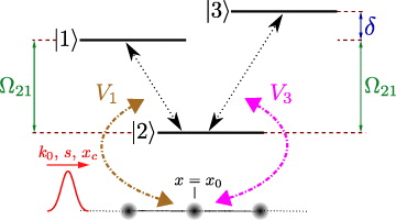
Figure 1. The V-system consists of the ground state |2〉 and the two upper states |1〉 and |3〉. The transition energy between |2〉 and |3〉 is detuned by δ with respect to the transition energy between |2〉 and |1〉, denoted by Ω21. The waveguide mode couples from site x0 to the two atomic transitions with the strengths V1 and V3. The initial single-photon state is a Gaussian wave packet with width s, carrier wavenumber k0 and is centered around xc.
Download figure:
Standard image High-resolution imageAs a result, the Hamiltonians  , which describe the interaction of the waveguide modes with the (yet to be specified) 3LS are of the form

The sum in (3) runs over the two dipole-allowed transitions denoted by α and β. The states |l↓〉 and |l↑〉 represent the lower and upper states of the transition l, respectively. The coupling strengths to the waveguide modes are given by Vl. For simplicity, we assume that the coupling constants are independent of the wavenumber k, so that we obtain a local coupling of the 3LS to a single waveguide site x0 (cf the above discussion regarding the use of a tight-binding model for the waveguide).
The full Hamiltonian (1) commutes with the total number of excitations

As a result, the Hilbert space associated with the system waveguide + 3LS may be decomposed into subspaces of conserved excitation number. In turn, this facilitates the utilization of exact numerics as described below.
The second sum in (4) runs over all upper states |γ↑〉 of the impurity. In this work, we restrict ourselves to the transport of single photons through the waveguide + 3LS system, so that  . The most general single excitation state
  of our system reads

where the first sum runs over all waveguide sites x and over the lower state(s) |ξ↓〉 of the 3LS. We denote the corresponding photon occupation amplitudes of the waveguide sites x by  . Further, we denote with
  the occupation amplitude(s) of the upper impurity state(s) |γ↑〉 and there is no photon in the waveguide.
For dynamical transport calculations, we evolve an initial quantum state |Ψ(t0)〉 in time according to

In particular, we utilize a Krylov-subspace-based operator-exponential techniques [10, 14, 15]. In the following, we will exclusively work with initial states without the excitation of the upper atomic level(s), i.e.  in (5). For the initial photon amplitudes
  we employ a normalized Gaussian wave packet in one or two of the subspaces associated with the lower state(s) of the impurity. Observables for transmittance, reflectance and occupation of the atomic states are defined in analogy to earlier works [10, 14, 15].
3. Single-photon transport through undriven three-level system
We investigate the scattering of single photons by a 3LS that is coupled to a waveguide. To this end, we employ analytical calculations for stationary situations involving plane wave states (cf [9, 27]) and compare with numerical analyses that focus on the dynamical features of the systems (using the time-evolution technique described above, cf [10, 14, 15]).
3.1. Long-time occupation in an undriven V-system
The atomic Hamiltonian  and the interaction Hamiltonian
  for an undriven V-system read, respectively, as


Consequently, a general single-excitation state  and the initial state |Ψ(t0)〉 for an incoming single photon read, respectively, as


Here, the Gaussian wave packet  of width s and which is centered at xc is launched with wave vector k0 (corresponding to the photon energy k0; see also figure 1).
In figure 2, we display the occupation of the two upper atomic levels as a function of the simulation time t and the detuning δ, when the atomic transition is on resonance, i.e. Ω21 = k0. In these plots, pronounced tails occur and this indicates a long-time occupation of the upper levels. Numerical diagonalizations have revealed that this effect arises from the excitation of almost dark states, i.e. states with a high occupation of the upper atomic states and a very low but non-vanishing occupation of the waveguide. Such states are eigenstates of systems whose detuning δ is small but non-zero and where the carrier wavenumber's energy is on resonance with one of the two transitions. These characteristics can be understood as follows.
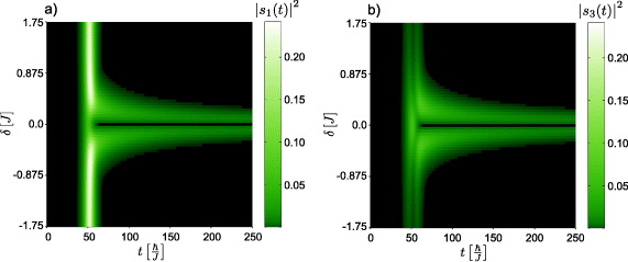
Figure 2. Occupation of the upper atomic states |1〉 (panel (a)) and |3〉 (panel (b)) for a simulation of a single-photon pulse of the form (10). The occupation is shown as a function of the simulation time t and the detuning δ of the two atomic transitions. Note the long-time occupation for small values of the detuning δ. The parameters of the simulation are V1 = V3 = J, Ω21 = k0, ω0 = 0, k0 = π/2, s = 9, xc = 400, and the waveguide has an extent of 999 real-space sites.
Download figure:
Standard image High-resolution imageInserting (9) into the time-dependent Schrödinger equation leads to the following equations of motion (we set E2 = 0 and x0 = 0 for simplicity):


and a slowly varying amplitude g0, i.e. ![$[\vert \partial /\partial t\, g_0(t)\vert]_{t=t_0}\!\!\! \ll \vert J\vert .$](https://content.cld.iop.org/journals/1367-2630/15/8/083019/revision1/nj469413ieqn17.gif) With the help of (11a), it then follows that
With the help of (11a), it then follows that

Inserting (13) into (11b) finally leads to


In other words, the emission of radiation from the atom into the waveguide is slow if the amplitudes of the upper atomic states follow (13) and if the detuning δ is almost vanishing. The first condition depends on the amplitudes and the relative phase of the upper atomic levels. The second condition is exactly the one mentioned above for which these almost dark states occur.
In the above argumentation, we did not allude to the amplitudes  . If the atom radiates into the waveguide, the sites at x ≠ x0 transport the radiation away from the atom. Effectively, these sites form a loss channel of a cavity (site x0) to which the atom is coupled. In this picture, a similar long-time occupation effect should occur in a poor man's model of a single 3LS interacting with a single mode of a leaky cavity. In this model, losses can be modeled by a negative imaginary part of the cavity's on-site energy. In the equations of motions (11a)–(11c) the waveguide part can then be formally replaced by

and we arrive at the poor man's model. Here, ωc denotes the cavity's on-site energy. A general single-excitation state  of this system is of the form

In figure 3, we display the occupation of the upper atomic levels in our poor man's model for the same parameter ranges as in figure 2. In these simulations, the single excitation initially occupied the cavity mode and the atom was in its ground state, i.e.  and
and  in (16). As expected, the characteristic tails associated with long-time occupations can be recovered qualitatively by our effective poor man's model system.
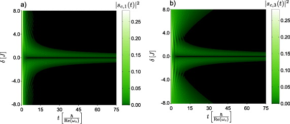
Figure 3. Occupation of the upper atomic states |1〉 (panel (a)) and |3〉 (panel (b)) for the simulation of a V-type three-level atom, which is coupled to a leaky single-mode cavity in the regime of a single excitation. The long-time occupation can occur in such systems, too. See text for further details. The parameters of the simulations are V1 = V3 = 2 Re(ωc), E1 = Re(ωc), Im(ωc) = −2.
Download figure:
Standard image High-resolution image3.2. Non-stationary dark states and phase-dependent scattering by an undriven Λ-system
The Hamiltonian  for the free and undriven Λ-system reads

while the interaction  of the waveguide modes with the atom is modeled by

and a general single-excitation state in this system is of the form

The undriven Λ-system thus exhibits two energetically lower states, |1〉 and |2〉. From each of these states the absorption of photons in conjunction with the transition to a (common) higher state |2〉 is possible. The details depend on the initial state of the atom and we consider here two possibilities. First, we look at the one-channel case (OCC), whereby the atom is initially in one of the lower states, e.g. without the loss of generality, in state |1〉. For this OCC, we use the initial state

The second class of initial states we consider here is that of a coherent superposition of the two lower atomic states—the two-channel case (TCC). The corresponding initial states read

Here, the relative phase  between the two lower atomic states is a new and, as we shall show below, important parameter. The setup of the corresponding simulations is shown in figure 4.
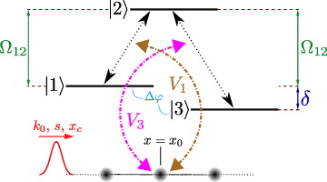
Figure 4. Illustration of waveguiding systems with a side coupled Λ-system. The notations are essentially the same as in figure 1. The only new parameter here is the relative phase Δφ between the two lower atomic states.
Download figure:
Standard image High-resolution imageAs usual, inserting (19) into the time-dependent Schrödinger equation leads to the equations of motion for this system (E1 = 0,x0 = 0):


3.2.1. Non-stationary dark states
In a dark state, the upper atomic state |2〉 will always be unoccupied, i.e.  . With the help of (22c), this leads to g1,0 = −V3/V1 g3,0 and, by employing (22b) and (22a), we obtain


If the coupling of the waveguide to both atomic transitions is equal, i.e. V1 = V3 and Δφ = π, the system is in a non-stationary dark state. An example for this case is shown in figure 5.
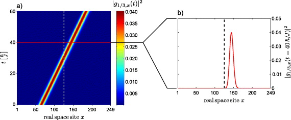
Figure 5. Occupation of the waveguide sites as a function of time (panel (a)) and a snapshot (panel (b)) when the photon has completely passed the waveguide site to which the three-level quantum impurity is side coupled to (indicated by a dashed line). The figure displays only one of the two channels since the occupation is identical in both. The wave packet is transmitted completely, i.e. the system is in a non-stationary dark state, although the photon energy k0 is on resonance with the transition energy Ω12. The parameters of the simulation are Δφ = π, V1 = V3 = J, Ω12 = k0, δ = 0, k0 = π/2, s = 7, xc = 65, and the waveguide consists of 249 real-space sites.
Download figure:
Standard image High-resolution image3.2.2. Phase dependence in the degenerate case
The above raises questions regarding the properties of stationary scattering solutions. As usual, we employ a time-harmonic ansatz for (22a)–(22c)

where Ek represents the eigenenergy of a stationary solution. The amplitude wj,x describes an excitation of the waveguide site x in channel j, i.e. in the subspace of the atomic state |j〉. To arrive at the stationary scattering solutions for a TCC, we make the ansatz
 , is scattered by the Λ-system into a reflected and a transmitted part in channel 1 (r11 e−ik11x and t11 eik11x in (27a)) and into a reflected and a transmitted part in channel 3 (t31 eik31x and t31 e−ik31x in (27b)). By the same token, the incoming plane wave in channel 3, i.e.
  , is similarly scattered into both channels (channel 3: r33 e−ik33x and t33 eik33x in (27b), channel 1: t13 eik13x and t13 e−ik13x in (27a)).
The wavenumbers in each of the distinct scattering process above are related via


Now, we assume that before any interaction of the photon and the atom takes place, the combined system of waveguide and atom is in a product state of waveguide modes with atomic states. In this case, the wavenumbers that describe the incoming photon cannot be different for the two atomic subspaces, i.e. we have

Under these conditions our ansatz reads


The physical interpretation of these coefficients is as follows. Initially, we have a degenerate Λ-atom in an equal superposition of its lower states, i.e.

Then, a single photon with wavenumber k is scattered by the atom. After the scattering, we detect the photon as either being reflected or transmitted. In the first case, the state of the atom after scattering is

In the second case, the state of the atom after scattering is

In figure 6, we display the transmittances  and reflectances
  for each channel
  according to (32a)–(32d). Furthermore, we depict in figure 6 the absolute deviations to the corresponding values of
  and
and  that we have obtained from Gaussian wave packet simulations of (21). Here, we have chosen equal coupling strengths V1 = V3 = J, so that the reflection amplitudes (32a) and (32c) are identical. Therefore, if a reflected photon is detected, the relative phase factor
  in (33) becomes unity. This results in an equal superposition of the two lower atomic states which are then in phase.

Figure 6. The degenerate Λ-system for TCC initial conditions: calculated transmittance in channel 1 (panel (a)), channel 3 (panel (b)) and calculated reflectance in both channels (panel (c)) as a function of the relative phase Δφ and the detuning between the photon energy k and the transition energy Ω12. In contrast to the transmittances, the reflectances in each channel are identical for all parameters. Panels (d)–(f) show the absolute difference of the analytical stationary solutions and the results of time-dependent simulations for Gaussian pulses as described in figure 5. For Δφ = π, this difference vanishes completely. This situation corresponds to the case of time-dependent dark states mentioned in the text. Generally, the simulated results for the transmittances and the reflectances differ due to the finite width in momentum space of the pulse. The parameters of the simulation are V1 = V3 = J, Ω12 = 0, δ = 0, k0 = π/2, s = 9, xc = 85 and the waveguide consists of 299 real-space sites.
Download figure:
Standard image High-resolution imageAs a result of the atomic superposition being in phase, figure 6 demonstrates that now a second photon with k = Ω12 would be reflected completely—and this is independent of the energy of the first reflected photon. The atom acting as a perfect mirror is well known from similar systems where 2LS [9] or V-systems [27] serve as quantum impurities. However, as our above discussion demonstrates, for an undriven Λ-system, this behavior can only occur in a TCC.
If a transmitted photon is detected, figure 6 demonstrates that the resulting atomic state after scattering strongly depends on the initial relative phase in (33). Even though both transmittances  exhibit maxima, after scattering the atomic state remains in a superposition of both lower states.
4. Single-photon transport through driven three-level system
4.1. Transmittance through a driven Λ-system
The Hamiltonian of a free but driven Λ-atom in the rotating-wave approximation and in a co-rotating frame reads (cf [27] and figure 7)

Here, Δ is the detuning between the driving field and the energy of the driven transition. The Rabi frequency is denoted by ΩR. This Hamiltonian can be diagonalized, i.e.

with the new dressed states

and their corresponding eigenvalues are

Further, the effective Rabi frequency is denoted by

In this dressed-state basis, the interaction Hamiltonian  then reads as

where the new coupling strengths are

Obviously, equation (41) has the same form as (8). Thus, the side-coupled driven Λ-system in the dressed-basis representation maps onto an undriven V-system with eigenenergies E± and coupling strengths V± depending on the detuning Δ and the Rabi frequency Ωeff of the driving field (cf [27]). For a plane-wave state, the reflection coefficient r in the stationary regime is determined by

As calculated in [27] for a linearized dispersion relation, the reflection coefficient (43) vanishes in the case of two-photon resonance, i.e. k = Ω12 − Δ, which is also the case in the present system. In other words, this is a realization of EIT for a single photon and a single atom.
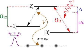
Figure 7. Illustration of the waveguiding system with a side coupled driven Λ-system. The transition between the states |3〉 and |2〉 is driven by a classical time harmonic electric field that couples to the transition with a strength described by the Rabi frequency ΩR. The frequency of the driving field is detuned to the transition energy by a value of Δ. The remaining notations are the same as those in figures 1 and 4.
Download figure:
Standard image High-resolution imageIn figure 8, we depict the analytically calculated reflectance |r|2 and a comparison to numerical simulations that use Gaussian single-photon pulses. For the pulses, the EIT effect is not as strong as it is in the case of a monochromatic plane wave, which again, is a result of the non-vanishing spectral width of the pulse.

Figure 8. Analytical transmittances |r|2 for plane-wave states with k = π/2 (panel (a)), corresponding simulated transmittances |rpulse|2 for a Gaussian pulse with k0 = π/2 (panel (b)), absolute difference between the simulation and the analytical calculation (panel (c)). The full transmittance (EIT) in case of the two-photon resonance (main diagonal in panel (a)) is not perfect in the simulation due to the finite spectral width of the Gaussian pulse. The parameters of the simulations are V =ΩR = J, Ω12 = k0, s = 9, xc = 420 and the waveguide consists of 999 real-space sites.
Download figure:
Standard image High-resolution image4.2. Momentum transfer in a driven V-system
Similar to the driven Λ-system, the Hamiltonian of a driven V-system reads in the rotating-wave approximation and in a co-rotating frame (cf [27] and figure 9)
The corresponding dressed eigenstates | + 〉 and | − 〉 are

and the new eigenvalues E+ and E− read

where the effective Rabi frequency Ωeff is identical to that of section 4.1. Consequently, the Hamiltonian  describing the interaction of the waveguide modes and the atom reads

where the coupling strengths are

Equation (47) is of the same form as (18). Hence, the driven V-system is mapped to an undriven Λ-system. As in section 4.1, the eigenenergies and coupling strengths depend on the detuning Δ and the Rabi frequency ΩR.
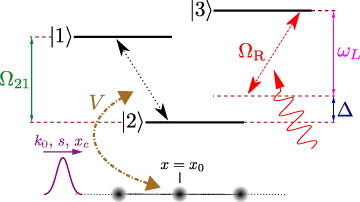
Figure 9. Parameters in systems with a side coupled driven Λ-system. The parameters are denoted in the same way as in figure 7.
Download figure:
Standard image High-resolution imageThe fact that a driven V-system effectively behaves like an undriven Λ-system implies that we need to consider all possible initial conditions of an undriven Λ-system, for instance, OCCs or TCCs. The two lower states of the mapped driven V-system are the states | + 〉 and | − 〉. In general, the initial state of the atom is a superposition of the states | + 〉 and | − 〉 in turn, this superposition can be controlled and prepared experimentally by techniques such as STIRAP [20].
In the following, we do not address the problem of the atomic state preparation and restrict our investigation to the OCCs. We assume that the atom, without the loss of generality, is initially in state | + 〉. According to (46), the two transition energies of the mapped Λ-system read

Let k+ be a wavenumber of a photon, which is absorbed in the channel of state | + 〉. Then, the wavenumber that corresponds to a photon scattered into the channel of state | − 〉 is determined by

This is a consequence of energy conservation. Upon combining (50) and (49), we obtain

where

The signs in (51) distinguish between the cases where k− belongs to either a transmitted (plus) or to a reflected wave (minus).
In figure 10, we display the dependence of k− on γ. If γ ⩽ − 1, k− is complex with a constant real part Re(k−) = π. In this case, the radiation emitted into the channel of state |3〉 cannot propagate in the waveguide, gets reabsorbed and emitted into the channel of state |1〉. Hence, the atom will be in state | + 〉 after scattering. This effect can be enhanced to an extreme by increasing the effective Rabi frequency Ωeff to Ωeff ⩾ 4J. In this case, the atom will stay in state | + 〉 after scattering independent of the wavenumber k+ of the incoming photon. This effect is attributed to the existence of band edges and band gaps in the dispersion relation of the waveguide and cannot occur in waveguiding systems whose spectrum is unbound.
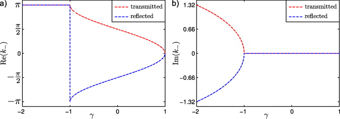
Figure 10. Real part (panel (a)) and imaginary part (panel (b)) of the wavenumber k− as a function of the parameter γ in (51). The red lines correspond to right moving and, therefore, transmitted waves, whereas the blue lines correspond to left moving and, therefore, reflected waves.
Download figure:
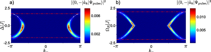
Standard image High-resolution imageIn figure 11, we display the photon's momentum distribution in the channel of state | − 〉, i.e.  , as a function of Δ and ΩR, respectively. The state |Ψpulse〉 is a Gaussian pulse of the form (20). The ladder operators
  in momentum space are related to those in real space via a lattice Fourier transform [10]. We clearly observe the region where the emission into the channel of state | − 〉 is forbidden—as noted above, this is a result of the finite bandwidth of the waveguide's dispersion relation.
Figure 11. Occupation of momentum space in channel ' − ' after scattering by varying the detuning Δ (panel (a)) and the Rabi frequency ΩR (panel (b)) of a time-domain simulation for a single-photon pulse and the corresponding wavenumbers calculated from (51) (white dashed lines). Note the cut off due to the finite bandwidth of the waveguide (red dashed lines). The parameters of the simulation are (a) ΩR = V =J, Ω21 = k0, k0 = π/2, s = 9, xc = 420 and (b) Δ = 0, V =J, Ω21 = k0, k0 = π/2, s = 9, xc = 420 and the waveguide consists of 999 real-space sites.
Download figure:
Standard image High-resolution image
5. Conclusion
In conclusion, we have investigated the single-photon transport properties in a 1D waveguide with an embedded three-level quantum impurity. In such systems, the wavepacket dynamics in the case of the V-type quantum impurity exhibits the striking feature of long-time occupations of the upper atomic levels. We have shown that this originates in the excitation of almost dark states in systems where the upper atomic levels are slightly detuned. Further, we have shown that this effect also occurs in a simplified poor man's model, where we have replaced the waveguide by a leaky cavity. Hence, this effect should be independent of the actual kind of waveguide the V-type quantum impurity is embedded in. In turn, this effect might, therefore, find applications in the field of all-optical buffers.
In contrast to a V-atom, a Λ-type three-level quantum impurity embedded in a waveguide supports non-stationary dark states. Furthermore, in the case of TCC and the impurity being in an equal superposition of its degenerate lower states, we have shown that the scattering characteristics depend strongly on the relative phase between these lower states. This may be exploited to characterize the fidelity of preparing a specific state of a 3LS with a prescribed relative phase.
For driven 3LS, we have found that a transmittance of unity due to an EIT of single photons cannot be fully realized by a single-photon pulse because of its finite spectral width. We have further shown how the finite bandwidth of a waveguide's dispersion relation influences the scattering properties of driven systems and how a change in the driving field's parameters affects both the quantum impurity's and the photon's states after scattering.
Acknowledgments
PL and KB acknowledge financial support by the DFG within the priority programme SPP Ultrafast Nanooptics (grant BU 1107/7-1).