


Abstract
Crystals of trapped atomic ions are among the most promising platforms for the quantum simulation of many-body quantum physics. Here, we describe recent developments in the simulation of quantum magnetic spin models with trapped 171Yb+ ions, and discuss the possibility of scaling the system to a level of complexity where classical computation becomes intractable.
Export citation and abstract BibTeX RIS
1. Introduction
Many-body quantum systems are often impossible to understand analytically and difficult to simulate numerically due to the exponential increase of required computational resources with system size. As Feynman proposed in 1982 [1, 2], a well-controlled quantum system could efficiently simulate another quantum system whose behavior is classically intractable. For example, a quantum simulator could be used to determine properties and dynamics derived from poorly understood models in condensed matter such as quantum magnetism [3], spin glasses [4], spin liquids [5] and high-temperature superconductors [6, 7]. Quantum spin models in particular can describe a large class of many-body quantum physics, and rich phenomena in condensed matter can be understood by finding the ground states of certain classes of spin Hamiltonians. Classical simulations of quantum spin models are currently limited to less than 40 spins [8, 9]; thus even quantum simulators of only 40 or more interacting spins are of great interest.
A quantum simulator can be viewed as a restricted version of a quantum computer, with quantum bits (qubits) playing the role of the spins. Compared to a quantum computer, a quantum simulator would not perform the universal computation, but could solve a certain difficult problem that is otherwise intractable. One way to operate such a quantum simulator is to borrow ideas from adiabatic quantum computation [10, 11], where the initial state of a non-interacting (trivial) Hamiltonian is adiabatically transformed to the corresponding ground state of the target Hamiltonian. Intriguing physics such as exotic magnetic order and quantum criticality can then be directly probed. Like quantum computers, quantum simulators require a platform with excellent coherence properties and controllable interactions, such as trapped atomic ions [12–21], neutral atoms [22–26], quantum dots [27] or superconducting circuits [28–30].
In this paper, we focus on the recent developments in the quantum simulation of the transverse Ising model with atomic ions confined to a linear chain. First we show how to realize effective spin–spin interactions and a transverse field with the trapped ion system (sections 2 and 3) [31]. Then we discuss the adiabatic algorithm and the criteria for the ground state evolution as it relates to the energy gap (section 4) [18]. In this general framework, we will show several results of the simulation such as a measured phase diagram (section 5) and a direct connection between spin frustration and entanglement with a small number of spins (section 6) [17, 18]. Finally, we present recent results on scaling the quantum simulation to larger numbers of spins (section 7) [19] and conclude with speculations on scaling the system approaching a level where classical modeling becomes intractable.
2. Realization of the transverse Ising model with trapped ions
The transverse Ising model for a set of interacting spin-1/2 particles is the simplest spin model that reveals interesting properties of quantum magnetism such as spin frustration and quantum criticality [32, 33]. Solving the Ising model in more than two dimensions and the transverse Ising model in two dimensions both belong to the class of 'NP-complete' problems [34–36] and thus can be related to a variety of intractable problems such as the traveling salesman problem [37]. The Ising model with a transverse field is described by the following Hamiltonian:

where σ(i)α, α = x,y,z, are the Pauli matrices of the ith spin, Ji,j is the Ising coupling matrix, By is an effective uniform transverse field and Planck's constant ℏ = 1 is assumed throughout.
Any two-level quantum system can be mapped to a spin-1/2 particle in an effective magnetic field. Atomic spins are typically represented by a pair of electronic or hyperfine levels [38–40]. In the work described here, the spin-1/2 system (denoted by  and
and  ) is represented by two hyperfine ground states of 171Yb+, 2S1/2
 and
and  , the so-called clock states separated in frequency by νHF/2π = 12 642 812 118 + 310B2m Hz. Here, F and mF
are quantum numbers associated with the total atomic angular momentum and its projection along a weak magnetic field of Bm ≈ 4 G. Note that the frequency difference of the clock state has only a small linear dependence on the external magnetic field, and coherence times exceeding 10 min have been reported in this atomic system [41]. In our experiment, the coherence time is measured to be of the order of 1 s without magnetic field shielding or compensation [42], which is much longer than the simulation duration, of the order of ms.
, the so-called clock states separated in frequency by νHF/2π = 12 642 812 118 + 310B2m Hz. Here, F and mF
are quantum numbers associated with the total atomic angular momentum and its projection along a weak magnetic field of Bm ≈ 4 G. Note that the frequency difference of the clock state has only a small linear dependence on the external magnetic field, and coherence times exceeding 10 min have been reported in this atomic system [41]. In our experiment, the coherence time is measured to be of the order of 1 s without magnetic field shielding or compensation [42], which is much longer than the simulation duration, of the order of ms.
Because atomic ions within a linear crystal are typically spaced by a few micrometers, the effective spins do not have sizable direct spin–spin interactions. Instead, large spin–spin couplings are induced by collective excitations of the vibrational normal modes through optical dipole forces. In the following, we discuss how to realize such spin–spin interactions in trapped ions intuitively (sections 2.1 and 2.2) and formally (section 2.3).
2.1. Quantum phases and harmonic motion
In the semiclassical limit of quantum mechanics, a particle is described by a wavepacket ψ, whose phase evolves according to

where L is the Lagrangian describing the dynamics of the particle along a particular path [43].
In a harmonic oscillator illustrated in figure 1(a), the Lagrangian is  , where m and ν are the mass of the particle and the natural frequency of the oscillator, respectively. The particle is resonantly excited when driven by an oscillating external force close to its natural frequency. When the external force F(t) = FA cos 2π(ν + δ)t is detuned from the frequency ν by δ ≪ ν, the particle trajectory and momentum are given by
and  , respectively, as shown in figure 1(b). Here the initial conditions are x(0) = p(0) = 0 and the particle returns to its initial position and momentum at τ = 1/δ. The trajectory in xp phase space is shown in figure 1(c). The obtained phase of the particle from equation (2) during τ is

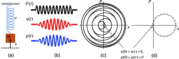
Figure 1. (a) A harmonic oscillator with particle mass m and natural frequency μ. (b) The response of the particle's position x(t) and the momentum p(t) when it is driven by an oscillating force F(t) = FA cos 2π(ν + δ)t, with x(0) = p(0) = 0. At τ = 1/δ, the coordinates x(t) and p(t) return to their initial conditions. (c) Phase space representation of the response, where the particle obtains the phase during the excitation by the amount of the action (equation (2)). (d) Phase space evolution of the response in a frame rotating at the natural frequency ν. The obtained phase is identical to the area of the closed space, and is sometimes called a geometric phase [44–46].
Download figure:
Standard imageThe area of the trajectory in the rotated phase space with frequency ν shown in figure 1(d) is identical to the value in equation (3) and is sometimes called a geometric phase. Note that the sign of the phase in equation (3) is directly related to the sign of detuning δ. If δ > 0, the driving frequency is larger than ν and the motion is out of phase with respect to the force. When δ > 0 (δ < 0), the system thus gains (loses) energy  with respect to the frame rotating at the harmonic trap frequency.
2.2. Spin-dependent forces and spin–spin interactions
An external driving force that depends upon the internal spin state generates a spin-dependent quantum phase. For multiple spins with collective motion, we find quantum phases that can depend non-trivially upon the collective spin states of the collection. Such phases can be interpreted as the result of an effective spin–spin interaction and can be used for quantum gate operations that generate entangled spin states. This type of interaction is central to the generation of the interacting spin models presented here.
The spin-dependent forces are classified according to which spin axis of the Bloch sphere diagonalizes the force, including σz-gate [44, 46] and σx,y-gate [47–50]. The σx-gates can be applied to clock states, whereas the σz-gate does not require high-frequency optical modulation techniques and can be less sensitive to optical phase errors. However, the principle of both types of operations is exactly the same, outside the spin basis. Here we first provide an intuitive explanation of the operation with a σz-force and later we present the formal description based on the σx,y-force.
A spin-dependent force can be realized through gradients of applied electromagnetic fields. For a spin state connected through a hyperfine transition, an oscillating magnetic field of amplitude B(x) having a detuning ΔB from spin resonance yields a potential V↑z = ± Ω(x)2/2ΔB on the  and
and  spin states as depicted in figure 2(a). Here the Rabi frequency Ω(x) = μBB(x)/2 parameterizes the dipole interaction of the spin with the field, where μB is the magnetic dipole moment for the spin system. The field B(x) can be implemented by a microwave field [51] or a pair of optical Raman fields coupling each spin off-resonantly to a third state through an electric dipole transition. In the latter case, ΔB is understood as the detuning of the beatnote of the two fields with respect to spin resonance. The force on the
  (
( ) state originates from the gradient of the applied field,
  (
( ), as shown in figure 2(b).
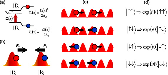
Figure 2. (a) The effective potential on a spin-1/2 system from an applied field detuned from resonance by ΔB. (b) A spin-dependent force from the intensity gradient of the applied field. Here F↑ = −F↓. (c) A spin-dependent force oscillating near resonance with the CM mode at frequency νCM, exciting only the CM motion for the states  and
and  . The CM motion correlated with the other spin states
  and
and  is not excited because there is no net force on the two-spin system. An oscillating force with frequency μ = νCM + δ can be generated by counter-propagating laser beams with a frequency difference μ. (d) Due to the excitation of the motion, the states
  and
and  will acquire a phase with respect to the other states
  and
and  as discussed in section 2.1. At τ = 1/δ, the collective motion is disentangled from the spin states, imprinting a phase Φ2 on
  and
and  .
.
Download figure:
Standard imageFor two ions in a harmonic trap, there are two collective vibrational modes in one dimension: the center of mass (CM) and stretch or tilt (TT) modes. We assume that an oscillating spin-dependent force on both spins is applied through the use of a 'walking standing wave' as shown in figure 2(c). When the frequency of this force is close to the CM mode, the CM motion will be excited for the spin states  and
and  . On the other hand, the spin states
  and
and  will not be influenced by the external force, since the two spins are pulled in opposite directions. As a result, the acquired phases depend on the spin configurations, as shown in figure 2(d). At τ = 1/δ, the collective motion returns to its initial position and momentum with the phase
  imprinted on the
  and
and  states. Note that the operation is equivalent to a quantum CNOT gate when Φ2 = π/2 [44, 46, 47].
At τ = n/δ (n = 1,2,3,...), the motional degree of freedom is disentangled from internal spin states and the evolution of the spin system at these times is exactly as though the system was influenced by the following pure spin Hamiltonian:

where F = F↑z = −F↓z,  , and we suppress constant offset terms in the Hamiltonian. The effective Hamiltonian (4) is exactly the Ising Hamiltonian for a two spin-1/2 system. By adjusting the sign of the detuning δ, the spin–spin interaction is controlled to be either ferromagnetic (FM) (δ < 0) or AFM (δ > 0). Note that this effective Hamiltonian only applies to those special times. However, this Hamiltonian is valid for all times in the limit
  , where the amplitude of actual motion x(t) (see section 2.1) is negligible.
The effective Ising interactions are generated through the collective motional mode excitation and the feature of the mode determines the characteristic of the Ising spin interactions. For three spins in a linear chain, in addition to the CM and TT modes we have zigzag (ZZ) mode. The eigenvectors of TT and ZZ modes are  and
and  , respectively. The effective Ising Hamiltonians through the motional couplings are then
where  ,
,  and δTT and δZZ are the detunings from the TT and ZZ modes, respectively. For the H(3)ZZ with a detuning δZZ > 0, the nearest-neighbor (NN) interactions (between spins 1 and 2 or spins 2 and 3) are FM, and the next-nearest neighbor (NNN) interaction (between spins 1 and 3) is AFM, with the NN interaction twice as large as the NNN interaction.
In principle, we can use the longitudinal and transverse vibrational modes to generate the effective Ising-spin interactions. We focus on the transverse modes because they are at higher frequencies for a linear crystal and can be more easily prepared near the ground state and suffer from less motional heating [52]. Moreover, the spectrum of transverse normal mode frequencies can be controlled through the anisotropy of the trapping potential [53], allowing more flexibility in setting the relative strengths of each normal modes' contribution to the effective Ising couplings. For example, we can control the relative strengths between NN and NNN interactions by adjusting laser detuning between the TT and ZZ modes. From equation (5), the NNN interaction dominates when tuned near the TT mode, while the NN interaction takes over when tuned closer to the ZZ mode.
2.3. General and formal descriptions of the Ising interaction
In the experiments reported here, the spin-dependent force is generated by the scheme proposed by Mølmer and Sørensen [48, 49]. The scheme produces differential forces on the spins in the rotated x basis of the Bloch sphere, where  and
and  . Unlike the σz-dependent force discussed in section 2.2, the σx-dependent force can be applied to magnetic-field-insensitive 'clock' spin states [47, 54, 55]. The Mølmer–Sørensen scheme applied to hyperfine ground states employs two pairs of non-copropagating laser beams with beatnote frequencies νHF
± μ. When the spins are simultaneously addressed by laser beams with equal intensities and coupled to the N transverse vibrational modes (νm, m = 1,2,...,N) along the x-direction, the resulting interaction Hamiltonian is
. Unlike the σz-dependent force discussed in section 2.2, the σx-dependent force can be applied to magnetic-field-insensitive 'clock' spin states [47, 54, 55]. The Mølmer–Sørensen scheme applied to hyperfine ground states employs two pairs of non-copropagating laser beams with beatnote frequencies νHF
± μ. When the spins are simultaneously addressed by laser beams with equal intensities and coupled to the N transverse vibrational modes (νm, m = 1,2,...,N) along the x-direction, the resulting interaction Hamiltonian is

where Ωi is the two-photon spin-flip Rabi frequency, σ(i)x is a Pauli spin-flip operator on spin i, and a†m and am are the phonon creation and annihilation operators for the harmonic normal mode m at frequency ωm. The Lamb–Dicke parameters  include the normal mode transformation matrix bi,m of the ith ion with the mth normal mode [56], and m is the mass of a single ion.
The time-evolution operator, UI(t), of the interaction Hamiltonian can be calculated by using the Magnus expansion
where ![$\hat {D}(\alpha \hat {O})= \exp [(\alpha ^* a-\alpha a^{\dagger })\hat {O}]$](https://content.cld.iop.org/journals/1367-2630/13/10/105003/revision1/nj396599ieqn40.gif) is the displacement operator and
is the displacement operator and

and

When the optical beatnote detuning μ is close to a particular normal mode νm, the spins become entangled with the motion through the spin-dependent displacement. At certain times, the final displacement α ≈ 0 and the motion nearly factorizes, which is useful for the quantum logic gates of synchronous entanglement between the spins as discussed in section 2.2 [45]. When the optical beatnote frequency is far from each normal mode compared to that mode's sideband Rabi frequency (|μ − νm| ≫ ηi,mΩi), the phonons are only virtually excited as the displacements become negligible (αm ≪ 1), and the result is a nearly pure Ising Hamiltonian for all times from the last (secular) term of equation (7),

where

When |μ − νm| ≫ δν for all modes m, where δν is the frequency spread of all modes, the strength of Ji,j follows a dipolar decay pattern in space 1/|i − j|3 [12, 13]. When the laser beatnote detuning μ is close to a single motional mode νm compared with the other modes, various long-range interaction patterns emerge that mimic the product of the eigenvectors of that particular normal mode on each ion. For example, when tuned near the second-to-highest (TT) mode of a linear crystal, the first and last ions in the chain interact most strongly, even though they are the furthest apart in space.
In the adiabatic state evolution, where we work with an additional transverse field added to the Ising model, the above analysis is more complicated. But in the limit where the phonons are only virtually excited and their occupancy is always small, the extra complication comes only from the fact that the spin Hamiltonian in equation (8) is modified by an additional transverse field term with a time-dependent magnetic field.
2.4. Extensions of the spin–spin interaction
With the same trapped ion system, higher-dimensional spin systems can be realized, depending on the details of the internal states in the atomic species. For example, a spin-1 system can be represented by the three Zeeman states in 2S1/2 F = 1 of 171Yb+, the  ,
,  and
and  states uniformly separated in frequency by the linear Zeeman splitting νzm. In this case, a pair of Raman laser beams with σ+ and π polarization with the beatnote frequency of νzm can result in the rotation operator Sx operation of the spin-1 system. Similarly, changing the phase between the laser beams will result in the Sy operation.
When bichromatic laser beatnote frequencies are detuned by ±μ from the resonant transitions νzm similar to above, a spin-dependent force is generated on the spin-1 system. The Hamiltonian from the force is similar to that of equation (6), replacing σx with Sx. As shown previously in equation (7), this spin-dependent force on the spin-1 system provides an effective S2x interaction. The end result is a spin-1 Ising Hamiltonian of equation (8). Here, we neglect the second-order Zeeman shift, since it can be compensated for either by taking a proper rotating frame on  or by adding a non-resonant compensation laser beam.
The Ising coupling scheme above can also be extended to act on multiple components of spin operators in order to simulate spin Hamiltonians such as the 'XY ' model  and the more general anisotropic Heisenberg spin model
  .
.
These spin models can be realized by adding one or two more pairs of laser beams in different directions [12] or by utilizing different frequency ranges. For example, the σyσy interaction term can be achieved by changing the phase of bichromatic Raman laser beams where beatnote frequencies are detuned near the vibrational modes along the y-axis. The σzσz interaction can be realized by applying the Raman beatnote detunings set to nearly half of the motional sideband frequencies μ ≈ νm/2 [57, 58]. In this condition, the spin-dependent force on the σz operation is the dominant term in the time evolution described by the following effective Hamiltonian:

where Ωeffi = Ω2i/2μ. As we discussed, the σz-dependent Hamiltonian (10) generates the σzσz-type spin–spin interactions.
3. Experimental demonstration of the Ising interaction
We trap 171Yb+ ions in a three-layer linear rf-Paul trap [59], with the nearest trap electrode a transverse distance of 100 μm from the ion axis shown in figure 3(a). An rf potential of amplitude ∼200 V at 39 MHz is applied to the middle layer, and the top and bottom layers are segmented into axial sections, where static potentials of the order of 10–100 V are applied for axial confinement. The ions form a linear chain along the trap Z-axis, and the axial CM trap frequency is controlled in the range νz = 0.6–1.7 MHz. In the transverse X-direction, the highest frequency normal mode of motion is the CM mode, set to about ν1 ≈ 4 MHz. The second highest is the TT mode at frequency  , where the trap anisotropy ε = νz/ν1 ≪ 1 scales the spacing of the transverse modes. For three ions, the lowest ZZ occurs at frequency
  . The other transverse Y -modes are sufficiently far away from the X-modes and do not overlap. Moreover, the coupling to these modes is suppressed by a factor of >10 by rotating the principal Y -axis of motion to be nearly perpendicular to the laser beams.

Figure 3. (a) Schematic representation of the ion trap apparatus and the geometry of Raman laser beams for the spin-dependent force. Two Raman beams uniformly address the ions, with Δk along the transverse x-direction. The spin states are defined with respect to a magnetic field of ∼4 G along the y-axis, and because the laser beams are each linearly polarized and perpendicular to each other in the xz-plane, the Raman transitions are driven between states as shown in (b). A photomultiplier tube (PMT) and charge-coupled-device (CCD) camera are used to measure the spin state of each ion through standard spin-dependent fluorescence. (b) The spin-1/2 system is represented by  and
and  in the S1/2 manifold in 171Yb+. The Raman laser beams are detuned by Δ from P1/2 states and induce coherent Rabi oscillations. When the Raman beatnote frequency is tuned to match the spin state frequency splitting νHF, the laser coupling generates the effective transverse field in equation (1). When the beatnote frequencies are detuned ±μ from νHF, the laser coupling generates the spin-dependent force and effective Ising couplings as discussed in the text.
Download figure:
Standard imageWe direct two Raman laser beams onto the ions to drive spin-dependent forces, with their wavevector difference aligned along the transverse x-axis of ion motion ( , where k = 2π/λ) (figure 3(a)). The Raman beams are detuned 0.5–2.7 THz to the red of the 2S1/2–2P1/2 transition at a wavelength of λ = 369.76 nm shown in figure 3(b). The Raman beams are phase modulated at a frequency nearly half of the 171Yb+ hyperfine splitting with a 6.32 GHz resonant electro-optic modulator, and each of the two Raman beams have independent acousto-optic frequency shifters in order to select appropriate optical beatnotes to drive Raman transitions [60]. The Raman beams are focused to a waist of approximately 30–100 μm with a power of up to 10–20 mW in each beam. When their beatnote is adjusted to drive the carrier transition at the hyperfine transition νHF, we observe a carrier Rabi frequency of Ωi/2π ≈ 1 MHz. For the spin-dependent force, we set Ωi/2π ≈ 0.4 MHz for each pair of Raman beams and for the transverse field, Ωi/2π is less than 0.1 MHz. The resonant transition generates the effective transverse field by adjusting the phase with respect to the spin-dependent force. For up to nine ions in a chain, we observe that the outer two ions experience ∼2% lower Rabi frequency and variation in the differential ac-Stark shift in each qubit of <1%.
In the experiment, we first Doppler laser cool 171Yb+ ions for 3 ms using a laser tuned to the red of the 2S1/2–2P1/2 transition at a wavelength of 369.53 nm. We then Raman sideband cool all m modes of transverse motion along x to mean vibrational indices of  in about 0.5 ms, well within the Lamb–Dicke limit. Next, the ions are each initialized to the
  state through standard optical pumping techniques [42]. We then apply the optical spin-dependent force on the ions for a duration τ by impressing the bichromatic beatnotes at νHF ± μ. Afterwards, the spin states are measured by directing resonant laser radiation having all polarizations on the 2S1/2(F = 1)–2P1/2(F' = 0) transition following standard state-dependent fluorescence techniques [42]. We use a CCD imager (the detection efficiency is 95% per spin). We determine the probability of each spin configuration (for example P↑↑↓ ) by repeating the above procedure more than 1000 times. We also measure the probability Pn of having n spins in state |↑〉 by using the PMT, which is useful for higher-efficiency measurements of certain symmetric observables such as entanglement fidelities and witness operators.
3.1. The two-spin case
Figure 4(a) shows the theoretical values of J = J1,2 from equation (9) and measurements at various detunings μ for two spins with  , where
  and
and  are the Lamb–Dicke parameters for CM and TT modes. The solid theoretical curve is plotted with no adjustable parameters, as the motional mode frequencies and the sideband Rabi frequencies are independently measured.
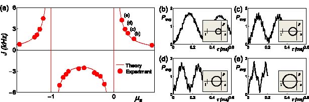
Figure 4. (a) Measured coupling J for two ions as a function of detuning μ overlaid with theory (lines) from equation (9) with no free fit parameters. The detuning is scaled to the axial (νz) and transverse (ν1) CM normal-mode frequencies of motion such that CM and TT modes of transverse motion occur at μS ≡ (μ2 − ν21)/ν2z = 0 and −1, respectively. (b) Time evolution of the average number of ions in the  state under the influence of the bichromatic force in the far-detuned limit, showing the secular oscillation of the Ising spin–spin coupling, where the detuning μ/2π is 80 kHz from the CM motional sideband. (c) Measurements with
  . Here the small oscillations from the motional excitation and the coupling to spin states are noticeable on top of the sinusoidal oscillations of the Ising interactions. (d) Measurements at
  . (e) Measurements at μ − ν1 = 2η1Ω/2π ≈ 32 kHz. The insets of panels (b)–(e) show the respective wavepackets in phase space and the areas enclosed are shaded.
Download figure:
Standard imageWe measure the strength of J by observing the time evolution between  and
and  after applying the spin-dependent forces on
  states. The evolution for the two spins is simply described by
  when we neglect the couplings between internal states and the motion. As shown in figure 4(b), the oscillations of the populations are sinusoidal, with frequency 2J. To detect the sign of the Ising coupling, we applied the same force on the initial state
  and observe the phase of the oscillations.
When the beatnote detuning μ is close to a vibrational mode, or |μ − ν1,2| is within a few sideband linewidths η1,2Ω, the coupling between motion and spin states modulates the spin state evolution. Figure 4(e) shows the spin state evolution at a detuning δ = μ − ν1 = 2η1Ω [48]. In this case, the motional state is displaced in phase space by not more than |α| = 1, and at particular times during the evolution τ = n/δ (n = 1,2,...) the motional degree of freedom is decoupled from the internal state, enabling the generation of pure spin–spin entanglement. As the detuning δ increases as shown in figures 4(b)–(d), the maximum displacement decreases and the evolution approaches a pure sinusoid indicative of pure spin–spin interactions. Typical experiments are performed with δ ⩾ 4ηΩ, where the largest displacements |α| < 1/4, resulting in a 2% modulation of the spin evolution.
3.2. The three-spin case
For three spins addressed uniformly with the Raman laser beams, we have J1 = J1,2 = J2,3 as the NN interaction and J2 = J1,3 as the NNN interaction as shown in figure 5(a). Since the bandwidth of the transverse mode spectrum is relatively small, all modes can be addressed from a single laser beatnote and the signs and strengths of J1 and J2 are under great control as shown in figure 5(a) and equation (9) [31]. In the region μ > ν1, both have AFM interactions (J1,2 > 0), and in the region ν2 < μ < ν1, both have FM couplings (J1,2 < 0). In the region ν3 < μ < ν2, the NN interaction is FM (J1 < 0) and the NNN is AFM (J2 > 0). When μ is near the TT mode, J2 overpowers J1, and when μ is closer to the ZZ mode, J1 is stronger than J2. Finally, for μ < ν3, all interactions are FM again.
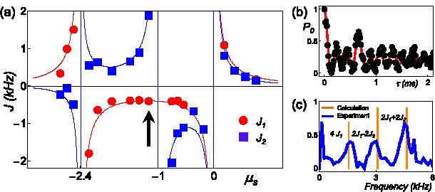
Figure 5. (a) Measured couplings J1 = J1,2 = J2,3,J2 = J1,3 for three ions as a function of detuning μ overlaid with theory (lines) from equation (9) with no adjustable parameters. At the scaled detuning μS, CM, TT and ZZ modes of transverse motion occur at μS ≡ (μ2 − ν21)/ν2z = 0,−1 and −2.4, respectively. (b) Time evolution of the probability P0 of all spins  under the bichromatic force in the far-detuned limit. Here, the two couplings J1 and J2 are clearly visible. The solid line is a fit to the time evolutions of equation (8) with an empirical exponential decay. The measurements are carried out at the indicated detuning in (a), or −50 kHz from TT mode. (c) The Fourier transform of the experimental curve shown in (b), where three peaks originate from the frequency components of 4J1, 2J1 − 2J2 and 2J1 + 2J2. The orange bars represent the calculated values from equation (9). The peak near the origin comes from the overall decay of the oscillation due to decoherence with ∼100 Hz.
Download figure:
Standard imageWe measure the J1 and J2 couplings by observing the oscillations in the population of state  after applying a spin-dependent force on the three spins. This population oscillates as cos2J1t cos J2t − i sin2J1t sin J2t, as shown in figure 5(b). We use Fourier analysis on the oscillations and find certain frequency combinations of the couplings 4J1, 2(J1 − J2) and 2(J1 + J2), as shown in figure 5(c). In this figure, we use theoretical values for the signs of J1 and J2.
In principle, we can produce an arbitrary spin–spin interaction graph with a linear string of trapped ions. For N spins, there are N(N − 1)/2 unique interactions that must be controlled independently. Instead of uniformly illuminating the ions with a single Raman beatnote, we can apply N different beatnote detunings to the ions, with a different power spectrum in each of these detunings for each of the N ions:

Here we can choose N2 different values of Ωi,k, which allows the possibility of full independent control of the sign and strength of all spin–spin interactions.
4. Adiabatic quantum simulation
In order to use the above spin–spin interactions to determine the ground state of a particular Hamiltonian, we adiabatically evolve from a trivial Hamiltonian to the one under study [61]. This approach is motivated by the adiabatic quantum computation algorithm first proposed as a method to solve NP-complete satisfiability problems [10]. The process of quantum adiabatic computation works as follows: a quantum system is initialized to the ground state of a trivial Hamiltonian. Next, the Hamiltonian is adiabatically deformed into the Hamiltonian of interest, whose ground state encodes the solution of a problem that has been mapped to the final Hamiltonian. If successful, the system will remain in the ground state and can be directly probed once the system arrives at the desired Hamiltonian. For quantum simulation of magnetically interacting spins, this approach allows the determination of ground states where the Hamiltonian can easily be written, yet the spin ground state cannot always be predicted, even with just a few dozen spins [9]. In this section, we describe the adiabatic quantum simulation of the transverse Ising model with three spins, where the exact solution is known, and discuss the criteria for adiabaticity. We then present experimental results for two example Ising interaction strengths and signs.
4.1. Basic principle of adiabatic evolution
We consider three Ising spins, where the transverse Ising Hamiltonian (1) is reduced to

This is the simplest Hamiltonian wherein the minimum energy state can exhibit frustration due to a compromise between the various Ising couplings. Additionally, the ground state phase diagram has a first-order transition as the Ising couplings are varied. As with the two-spin case, the non-commuting operators in the Hamiltonian can give rise to a quantum phase transition (QPT) in the thermodynamic limit.
We can calculate the exact instantaneous energy spectra as a function of the scaled transverse field By/|J1| for the Hamiltonian (equation (12)). In figure 6, we present two cases where the NN interactions are FM (J1 < 0), and examine the effect of changing the sign of J2. We will compare the adiabatic requirements for the following experimental trajectory. In all simulations the spins are initially prepared in the ground state of the transverse field (By ≫ |J1|), depicted by the solid circle (figure 6). The goal is to subsequently adiabatically lower the field compared to the Ising couplings. When By/|J1| ≪ 1 the Ising interactions determine the form of the ground state (for simulation details, see figure 7).

Figure 6. Energy level diagrams for equation (12) with two different types of spin–spin interactions. For both panels, the NN interactions are FM (J1 < 0). (a) The NNN interaction is FM with J2/|J1| ∼ − 2 and (b) AFM with J2/|J1| ∼ 0.9. The arrow in both diagrams indicates the trajectory in the simulation, initialized at By/|J1| ∼ 10. Under this condition, the initial ground state is an eigenstate of the second term in equation (12), a polarized state along By. In both examples, at B ≈ J1 some high-energy states cross, but the ground state (black solid line) has no level crossings with any excited state. Likewise, the highest energy state does not cross any other levels, allowing one to also adiabatically follow this state. The dotted lines represent excited states, which are most strongly coupled to the ground state along the path. In the large-field limit, the energy difference between ground and excited states Δge (here, scaled by  ) is proportional to By, but as By/|J1| decreases the spin–spin couplings determine the energy difference and the form of the ground state. In both (a) and (b), the final ground state is FM (defined along the x-axis of the Bloch sphere); however, in the case of (a), the minimum Δge is ∼20 times larger.
Download figure:
Standard image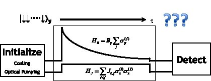
Figure 7. After preparing the spins in the ground state of  , we apply the Hamiltonian (1) with the condition of By(t = 0) ≫ Ji,j. Then we adiabatically reduce the strength of the transverse field By(t) to the final value By(τf), where Ising interactions are dominant. At various times along the path we halt the experiment and detect the spin states, thus mapping out the ground state phase diagram of Hamiltonian (1).
Download figure:
Standard imageIn figure 6(a), the NNN interaction is also FM (J2 < 0). There are no level crossings with the ground state (solid black line) over the trajectory indicated by the arrow; thus if the evolution of the Hamiltonian is sufficiently slow, excitations will be minimized. We can also change the sign of By and adiabatically follow the highest excited level, as it does not exhibit any level crossings.
In figure 6(b), J2 > 0 and the NNN interaction is AFM. The gap at the crossover to magnetic order determined by the Ising couplings is ∼15 times smaller than that of figure 6(a), requiring a slower change of By/|J1| to remain in the ground state. This gap is comparatively smaller because the Ising couplings J1 and J2 have opposite sign and are nearly equal in magnitude. When this is exactly true at zero magnetic field, there is an energy level crossing due to the competition between the two Ising couplings. For larger spin systems this competition persists and gives rise to an interesting phase diagram as described in section 5.
The general requirement of adiabatic following along the Hamiltonian trajectory H(t) described above is characterized by the condition [61]

In this expression, the dimensionless quantity  ≡
≡  characterizes the coupling from the ground state
  to any excited state
  with energy gap Δge. In the context of this paper, we consider the dynamic requirements to maintain adiabaticity and therefore only transitions allowed by symmetry are considered. The parameter is small, of the order of unity for this simulation, but is peaked at a crossover in magnetic order, where the instantaneous eigenstates are most rapidly varying.
Assuming that the parameters are smoothly changing, it is clear that to remain adiabatic the bottleneck is crossing a region containing a small gap. For an infinite-sized system, the gap shown in figure 6(a) will vanish at the point of a QPT. Of course in this limit, crossing a phase transition will lead to the formation of defects [62] and one needs to consider adiabaticity in the context of an acceptable level of excitations, as well as quantify how those excitations decay. For a finite-sized system it is instructive to consider the onset of a phase transition and the rich dynamics which can be studied. Although the minimum energy gap between two instantaneous energy levels will certainly be different depending on the form of the Ising couplings, for all cases of the generalized form of the Hamiltonian shown in equation (12), the adiabaticity criteria will be satisfied if the time to sweep through the gap is much larger than the inverse gap.
More specifically, equation (13) states that to remain adiabatic with respect to spin flip excitations, the rate of changing the time-dependent By-field profile must be shallow when the gaps in the energy spectrum are small (as in figure 6(b)), in particular near a crossover (corresponding to a phase transition for large N).
4.2. Experiments
We experimentally investigate this adiabaticity criterion for the two different types of NNN coupling that were introduced above. We initialize the spins along the By-direction through optical pumping (∼1 μs) and a π/2 rotation about the −x-axis of the Bloch sphere. Figure 7 shows the adiabatic simulation protocol. The simulation begins with a simultaneous and sudden application of both By and J1, J2, where By overpowers J1 (By/|J1| ≈ 10). A typical experimental ramp of By decays as By(t) = a e−t/τ + b with a time constant of τ ∼ 30 μs, varying from a ∼ 10 kHz to a final offset of b ∼ 500 Hz after t = 300 μs. By varying the power in only one of the Raman beams, this procedure introduces a change in the differential ac-Stark shift of less than 2 Hz. We turn off the Ising interactions and transverse field at different By/|J1| endpoints along the ramp. We then measure the magnetic order along the x-axis of the Bloch sphere by first rotating the spins by π/2 about the y-axis and detecting the z-component of the spins.
In figure 8(a) all interactions are FM and J2/|J1| ∼ − 2 (as in figure 6(a)). The dashed line is the adiabaticity parameters from equation (13) calculated over the trajectory for the two coupled excited states (recall figure 6). Due to the 500 Hz final offset of By, the simulation stops at By/|J1| ∼ 0.5. To examine the behavior below this value, we calculate the criteria for an exponential ramp with a 100 μs time constant. This profile was chosen to overlap with experimental parameters for large By/|J1| and also reach By = 0 in a typical simulation time (∼300 μs). The results indicate that equation (13) is satisfied over the trajectory;  remains much less than one even with a maximum occurring at By/|J1| ∼ 1. To demonstrate that the simulation is indeed adiabatic for these parameters, we plot the measured probability of occupying an FM state P(FM) = P↑↑↑ + P↓↓↓ (solid dots in figure 8(a)). The black line represents the adiabatic ground state and the grey line is the theoretical expected probability including the experimental ramp. The dotted line in this figure is the theoretical state evolution using a By-field ramp that reaches zero. The predicted evolution does not significantly deviate from the ideal ground state and the data are in good agreement with all three theory curves.

Figure 8. (a) The theoretical order from the exact experimental ramp with a 35 μs time constant and final offset value given in the text (gray solid line) is in reasonable agreement with the order in the true ground state (black solid line) for By/J1 > 0.5. The dotted line is the expected state evolution for a pure exponential decay ramp with a 100 μs time constant, allowing By → 0. (b) The data also match well to theory, as we avoided the regions where diabatic transitions are expected for By/J1 ≪ 1. According to calculations, the duration of three-spin experiments near the special point should be of the order of milliseconds.
Download figure:
Standard imageFigure 8(b) presents the case when the NNN interaction is AFM and J2/|J1| ∼ 0.9 (as in figure 6(b)). When By/|J1| ≪ 1,  reaches a maximum value of ∼0.6, indicating that the probability for excitations will likely increase. This difference is because in this case the gap Δge at the 'critical' point is ∼15 times smaller than that in figure 6(a). In contrast to the FM J2 case, the theoretical probability curve shown in figure 8(b) predicts significant diabatic effects when using this By-field profile for simulations near the critical point. In fact, to successfully evolve to the true ground state near By = 0, the simulation time (assuming the same initial conditions and an exponential ramp of By) should be at least a factor of ten longer.
Because all data lie outside the region where the energy gaps are small, the diabatic excitations are minimal, but further experimental study is needed to precisely quantify this effect. One method to probe excitations, which may also be useful as N ≫ 1, is to perform and then reverse the experimental ramp and measure the probability of returning to the initial state [62].
5. Phase diagram
Assuming adiabaticity as described above, we can generate an experimental phase diagram for the transverse Ising model. We will first describe this for the three-spin case, and then discuss specific features and scalability in sections 6 and 7. For the three-spin Hamiltonian in equation (12), the competition between the two spin–spin couplings and the transverse field gives rise to a rich phase diagram. Here, we label the 23 possible spin configurations as the two FM states,  and
and  , two symmetric AFM states,
  and
and  , and four asymmetric AFM states,
  ,
,  ,
,  and
and  , all defined along the x-axis of the Bloch sphere.
In figure 9(a), we plot a part of the theoretical phase diagram where the NN interactions are always FM (J1 < 0). The order parameter is the probability of occupying an FM state, P(FM) = P↑↑↑ + P↓↓↓. For regions where By/|J1| ≫ 1, the ground state is polarized along By with P(FM) = 2/2N = 1/4, as all states in the x-basis are equally populated and there are two FM states. As By/|J1| decreases, different magnetic phases arise. When the NNN interaction is also FM (J2 < 0), and By/|J1| ≪ 1 the ground states are the two degenerate FM states. In the region where the NNN interaction is AFM and J2 overpowers J1 (J2/|J1| > 1), the asymmetric AFM states are lowest in energy. A special point appears at J2/|J1| = 1 and By = 0, where all the contours of constant FM order meet. Here, the ground state will be a superposition of the FM and asymmetric AFM states. This effect arises because the pairwise interaction energy cannot be minimized individually, leading to a highly degenerate, or frustrated, ground state [17].

Figure 9. (a) Theoretical phase diagram for equation (12). The color scale indicates the amplitude of the FM order parameter,  . Here, J1 is always negative, yielding FM order in that coupling. In the region where J2/|J1| < 0, there is a crossover to FM order as By/|J1| is lowered. When J2/|J1| > 0, the AFM and FM interactions compete. When J2/|J1| = 1 and By = 0 the ground state is comprised of six states: four asymmetric AFM and two FM states. This creates a special sharpened point where all lines of equiprobable FM order converge. (b) Experimental measurements of the phase diagram for equation (1) (solid bars) compared to the theoretical prediction from figure 9 (surface). The vertical amplitude is the FM order parameter
  . The ratio of By/|J1| was varied from ∼10 to ∼0.1 for J2/|J1| values of −1.3, −2.0, −3.6, 4.2, 2.0, 1.3, 0.92, 0.74, and 0.62. J1 < 0 for all traces. (c) As By/|J1| → 0 in the region where J2/|J1| < −1, we observe a smooth crossover to FM order. The filled circles and solid line are the data and theory for J2/|J1| = −1.3, respectively. (d) When changing J2 for a fixed and small value of By/|J1| the system undergoes a sharp transition. The data (filled circles) shown are for a scan of By/Jy = 0.57. The average deviation per scan of By/|J1| from the exact ground state is ∼0.09.
Download figure:
Standard imageThis procedure is performed for nine different combinations of J1 and J2 determined by the beatnote detuning μ from equation (9). In figure 9(b) we present the results as a 3D plot of the FM order parameter, with the theoretical phase diagram (surface) from figure 9(a) superimposed on the data. The data are in good agreement with the theory (the average deviation per trace is ∼0.09) and show many of the essential features of the phase diagram. As By/|J1| decreases, a smooth crossover from a non-ordered state to FM order occurs in the region where J2/|J1| < 1 (figure 9(c)). The data (e.g. figure 9(c)) show small-amplitude oscillations in the initial evolution due to the sudden application of the spin–spin interaction, which is held constant during the simulation to minimize variation in the differential ac-Stark shifts. As the number of spins increases, this is an example of a QPT. A first-order transition due to an energy level crossing is apparent (figure 9(d)) when changing J2 for a fixed and small value of By/|J1| = 0.57. This transition is sharp even in the case of three spins [63].
6. Spin frustration and entanglement
We also study the properties of the ground states in the case of a frustrated Ising Hamiltonian. Frustration in spin systems occurs when spins cannot find a ground state that minimizes the energy of each pairwise interaction [3, 32]. As shown in figure 10(a), this can be simply illustrated by three spins with AFM interactions on a triangular lattice [64]. The situation gives rise to a large ground state degeneracy, leading to magnetic analogues of liquids and the crystal arrangement of ice [65, 66]. For quantum spins, the frustrated ground states are expected to be directly related to entanglement [67, 68].

Figure 10. (a) The simplest case of spin frustration in a triangular geometry with AFM interactions. (b) Image of three trapped atomic 171Yb+ ions in the experiment, taken with an intensified CCD camera. The spins in the linear ion string have NN (J1) and NNN (J2) interactions mediated by the collective vibrational modes. (c, d) Evolution of each of the eight spin states, measured with a CCD camera, plotted as By/Jrms is ramped down in time, with each plot corresponding to a different form of the Ising couplings. The dotted lines correspond to the populations in the exact ground state and the solid lines represent the theoretical evolution expected from the actual ramp, including non-adiabaticity from the initial sudden switch-on of the Ising Hamiltonian. (c) All interactions are AFM. The FM-ordered states vanish and the six AFM states are all populated as By → 0. Because J2 ≈ 0.8J1, a population imbalance also develops between symmetric and asymmetric AFM. (d) All interactions are FM, with evolution to the two FM states as By → 0.
Download figure:
Standard imageWe realize the textbook example of spin frustration in a unit triangular cell with AFM interactions by setting the Raman beatnotes μ to the blue side of CM mode. For comparison, we also study the ground state property of all FM interactions by setting μ to the red side of CM mode. Recall that a linear chain of three ions can have NN and NNN interactions through the collective normal modes as discussed in section 2 (figure 10(b)). The experimental procedure to prepare the ground states of the Hamiltonian with all AFM interactions and all FM interactions is the same as the description in section 4. Figure 10(c) shows the time evolution for the Hamiltonian frustrated with nearly uniform AFM couplings and gives almost equal probabilities for the six AFM states (three-quarters of all possible spin states) at By ≈ 0. Because J2 < 0.8J1 for this data, a population imbalance also develops between symmetric and asymmetric AFM states. Figure 10(d) shows the evolution to the two FM states as By → 0, where all interactions are FM.
The adiabatic evolution of the ground state of Hamiltonian (1,12) from By ≫ Jrms to By ≪ Jrms should result in an equal superposition of all classical ground states and therefore carry entanglement. For instance, for the FM case, we expect a GHZ ground state  . For the isotropic AFM case, we expect the ground state to be
  . We characterize the entanglement in the system at each point in the adiabatic evolution by measuring particular entanglement witness operators [69]. This is accomplished by performing various global rotations to the three spins before measurement and combining the results of many identical experiments. When the expectation value of such an operator is negative, this indicates entanglement of a particular type defined by the witness operator. For the FM case, we measure the expectation of the symmetric GHZ witness operator
  [50, 69], where
  is the identity operator and
  is proportional to the lth projection of the total effective angular momentum of the three spins. For the AFM (frustrated) case, we measure the expectation of the symmetric W-state witness,
  [69]. In both cases, as shown in figure 11, we found that entanglement of the corresponding form develops during the adiabatic evolution.
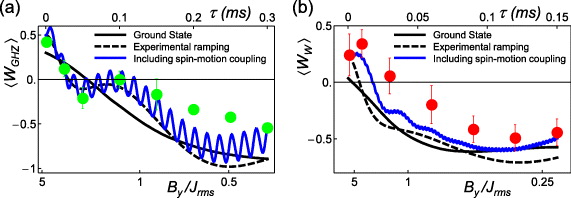
Figure 11. (a) Entanglement generation through the quantum simulation for the all FM interactions. We measure the entanglement by observing the expectation of a particular operator that indicates the presence of entanglement, called the entanglement witness [69]. For the case of all FM interactions, we use the Greenberger–Horne–Zeilinger (GHZ) witness [69], sensitive to the state  . We found that entanglement occurs when |By|/Jrms < 1. (b) Entanglement generation for the case of all AFM interactions. Here, we use the symmetric W-state witness, sensitive to the state
  and we find that entanglement emerges for By/Jrms < 1.1. In both (a) and (b), the error bars represent the spread of the measured expectation values for the witness, likely originating from the fluctuations of experimental conditions. The black solid lines are theoretical witness values for the exact expected ground states, and the black dashed lines describe theoretically expected values at the actual ramps of the transverse field By. The blue lines reveal the oscillation and suppression of the entanglement due to the remaining spin–motion couplings, showing better agreement with the experimental results. Note that the residual spin–motion couplings do not appear to impact on the FM order of each state, as shown in figure 10. In the theoretical curves we do not include other possible errors such as state detection inefficiency or errors due to spontaneous scattering or fluctuations in control parameters.
Download figure:
Standard imageIn macroscopic systems, the global symmetry in the Ising Hamiltonian (1) is spontaneously broken, and ground-state entanglement originating from this symmetry is expected to vanish for the non-frustrated FM case [33]. However, for the frustrated AFM case, the resultant ground state after symmetry breaking (e.g.  ) is still entangled. While spontaneous symmetry breaking does not occur in a small system of three spins, we can mimic its effect by adding a weak effective magnetic field
  to the Hamiltonian during the adiabatic evolution [18, 70]. We experimentally observed that the frustrated ground state carries entanglement even after global symmetry is broken by using an appropriate witness in the Ising model, and thereby establishes a link between frustration and an extra degree of entanglement [17].
As we discussed in sections 2 and 3, the spin degree of freedom is disentangled from the motion at discrete time steps, which results in pure spin–spin interactions. In the presence of transverse field, however, the disentanglement between motional states and spin states becomes imperfect and is accumulated during the adiabatic evolution. Fortunately, the residual entanglement does not have an influence on the probabilities of spin product states measured in the direction of the Ising model axis [71]. Therefore we do not see the effects on the experiments generating the phase diagram shown in section 5. The influence of spin–motion coupling becomes noticeable in the witness measurements, since the motional degrees of freedom are traced out during the spin state detections. As shown in the blue curves of figure 11, the entanglement of the spin states is suppressed because of the remaining spin coupling to motions.
7. Scalablility of the quantum simulation
As the number of spins N grows, the technical demands on the apparatus are not forbidding [17, 31]. In particular, the expected adiabatic simulation time for the spin models is inversely proportional to the 'critical' gap in the energy spectrum; for instance, in a fully connected uniform FM transverse Ising model in a finite-size system, this gap decreases as N−1/3 [72]. Scaling this system to accommodate long ion chains will allow the investigation of critical behavior depending on the the system size, which is intractable in classical numerical simulation.
We perform a benchmarking experiment where all interactions Ji,j are FM regardless of the number of spins in the system by tuning the Raman beatnote detuning close to the CM mode. We carefully investigate deviations of experimental simulations from theoretical predictions as the system size increases and discuss possible solutions overcoming the limitations. We observe a crossover from paramagnetic to FM spin order, and the crossover sharpens as the number of spins is increased, prefacing the expected QPT [33] in the thermodynamic limit. We found that particular order parameters of the system can be quite insensitive to the imperfections of the quantum simulations, and the extraction of intensive variables such as magnetization is much less susceptible to decoherence compared with full tomographic characterizations of the resulting quantum state.
In the experiment, we produce the strength of Ji,j close to 1 kHz by setting the Raman beatnote detuning μ ≈ ν1 + 4η1Ω, where ν1 are the Lamb–Dicke parameter and the frequency of CM motional mode, respectively. The strength of the couplings is pretty uniform among the pairs, since the CM mode dominates the interactions. The non-uniformity in the Ising couplings arises from other vibrational modes, which produce around 30% differences in the strength at most. We note that for larger detunings, the range of the interaction falls off even further with distance, approaching the limit Ji,j ∼ 1/|i − j|3 for μ ≫ ν1 [12, 13].
The experiment is performed according to the adiabatic quantum simulation protocol, as described in section 4 and shown in figure 7. We initially start with a strong effective transverse field By ≈ 5NJrms (N = 2,3,...,9) after preparing the ground state of the By Hamiltonian. We transfer it to the Ising Hamiltonian with a weak transverse field by exponentially ramping down By with time constant τ = 80 μs. We observe the evolution of state step by step as we proceed with the experiment. For the measurements, we use the PMT and obtain the probability Ps of having s spins in state  from a histogram of fluorescence counts, constructed by the more than ∼1000 × N times repetition of the experiments [73]. The final states of the adiabatic evolution are the superposition of two perfect FM states
  and
and  , called the GHZ state, since we implement FM couplings for all the pairs of spins and begin with the ground state of the transverse field. Therefore we measure the density matrix of the GHZ state as the simulation evolves. We also use other observables such as magnetization to characterize the time evolutions and the phase transitions.
We analyze the reliability of the simulation depending on the system size by using the fidelity of the GHZ state,  . Here P(FM) = P↓↓...↓ + P↑↑...↑ and the GHZ coherence |C↓↓...↓,↑↑...↑| is the coefficient of
  in the density matrix [50]. We measure the coherence of the GHZ state by observing the contrast of the oscillating parity signals (figure 12(b)), obtained by applying analysis π/2 pulse with different phases ϕ and taking the differences in population of the even number bright states and odd number bright states (P(0) + P(2) + ··· − P(1) − P(3) − ··· ).
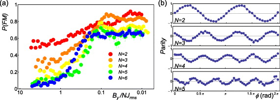
Figure 12. Experimental results of adiabatic quantum simulation depending on the system size. Here all pairs of spins have FM interactions. (a) The evolution of FM order parameter P(FM) as the system size increases. Initially P(FM) starts at 2/2N, since P(FM) is the probability of two states  and
and  over equally distributed 2N states. As the spin–spin interactions J overpower By (By → 0), P(FM) are developed. Here J is the average strength of all interactions. The red, orange, yellow, green and blue dots represent the experiments for the total number of spins N = 2, 3, 4, 5 and 6, respectively. Ideally P(FM) should be close to 1 at the end. However, P(FM) clearly reduces as the number of spins increases in the system from 2 to 6. The sources and amounts of errors are discussed in the text. (b) The parity oscillations for the final states of the simulation depending on the number of spins, obtained from the population difference between the even number of
  state and the odd number of
  state after applying analysis π/2 pulse and swiping its phase ϕ. The contrast of the oscillations provides the lower bound of the coherence, the off-diagonal element of the density matrix for the GHZ state
  . The coherences decrease to 0.8, 0.47, 0.35, 0.27 much faster than P(FM) as the number of spins increases from 2 to 5, because of spin–motional couplings during the simulation as discussed in the text.
Download figure:
Standard imageFigure 12 shows the experimental results of the quantum simulation as the number of spins increases in the system. Initially P(FM) starts 2/2N, since P(FM) is the total probability of two states ( ,
,  ) and the ground state of
  ,
,  is equally distributed in a total of 2N states in the x-basis. Ideally P(FM) should be close to 1 at the end of the simulation. However, we observe that the final states are increasingly deviating from the ideal situation as the number of spins grows as shown in figure 12(a). We also observe that the GHZ coherence decreases much more rapidly than P(FM) shown in figure 12(b). After six spins, we did not measure any significant GHZ entanglement for the final state due to the large suppression of the coherence compared to the populations. In the following subsections, we discuss the reason for these deviations and we summarize the expected experimental imperfections in quantum simulations as the system size grows.
7.1. Scaling of imperfections
7.1.1. Spin–motion coupling
As briefly discussed in section 6, the spin–motion entanglement does not completely vanish during the simulation; in contrast, the amount of coupling increases in the presence of the transverse field. The transverse field mixes the spin states along the axis where the spin-dependent force is applied; therefore this coupling induces phonon excitations, modifying the final state from the ideal GHZ state to  . Here
  is a motional coherent state and
  increases as the amount of state mixing grows. According to numerical calculations corresponding to the experiment,
  increases to ≈0.5 for the five-spin experiment. The effective phonon excitation occurs primarily in the early stages of the simulation evolution, where the strength of the transverse field is much larger than the frequency of spin rotations. In the experimental conditions, the Raman beatnote is detuned ∼4η1Ω from the CM mode, which results in an increment of |α|, because of the required large initial transverse field. However, the population P(FM) and the evolution is not sensitive to these spin–motion couplings.
7.1.2. Diabaticity
The finite ramping speed of parameters in the Hamiltonian leads to excitations out of the ground state and can lead to oscillations in the observed order parameter. This diabaticity in the evolution, along with errors in the initialization to the original ground state, is estimated to suppress the final value of P(FM) by ∼4% for N = 5 shown in the orange line of figure 13(a). As discussed in section 4, the diabaticity is related to the minimum gap over the trajectory of the Hamiltonian as well as the ramping time. We note that the gap between the ground and first excited state of the fully connected uniform FM model scales as N−1/3, implying that the simulation time increases by a factor of ten when the number of spins grows by a factor of 1000.
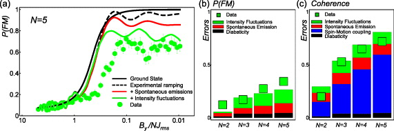
Figure 13. (a) Comparison of the experimental results of P(FM) to the theoretical expectations including various imperfections of experiments for the five spins. The black line represents the evolution of the perfect adiabatic evolution, and the dashed line shows the actual time evolution including the actual ramping of the transverse field with the imperfections of initial state preparations. The red line is obtained from the theory with spontaneous emissions and the green line is calculated by adding intensity fluctuations of 1.5%. The overall populations of P(FM) are in agreement with the green theoretical curve including all the above-mentioned imperfections. The horizontal shift By/J comes from the inaccuracy of the calibration that is not fully understood yet. (b) The amount of errors in P(FM) (the diagonal parts of the density matrix) from the ideal ground states for the cases of N = 2, 3, 4 and 5. (c) The amount of errors in coherence (the off-diagonal parts). In both (b) and (c), the green squares represent the total errors measured in the experiment and the bars illustrate the numerically estimated errors from the various sources of experimental imperfections. The black, red and green bars show the error amounts from non-perfect adiabatic evolutions, spontaneous emissions and intensity fluctuations. The blue bars stand for deviations from the spin–motion couplings shown in equation (7). The spin–motion coupling reduces the coherence significantly as the system size grows, while it does not have any influence on the P(FM).
Download figure:
Standard image7.1.3. Spontaneous emission
One of the major error sources is the spontaneous emission from Raman beams, which amounts to a ∼10% spontaneous emission probability per spin in 1 ms for a detuning of Δ ≈ 2.7 THz [74]. Spontaneous emission dephases and randomizes the spin state and thus introduces entropy into the system. In addition, each spontaneous emission event populates other states outside the Hilbert space of each spin with a probability of 1/3. Spontaneous emission errors grow with increasing system size, which also suppresses P(FM) order with increasing N, as seen in figure 13. We theoretically estimate the suppression of P(FM) due to spontaneous emission by averaging over quantum trajectories and solving density matrix equations to be ∼5% for N = 2 spins and ∼13% for N = 5 spins. The error contributions are the same for both populations and coherences.
7.1.4. Intensity fluctuations
Intensity fluctuations on the Raman beams during the simulation induce an ac-Stark shift on the spins. The ac-Stark shifts produce an imbalance in the blue and red sideband detunings, which give rise to the imperfection of spin–spin interactions. According to our numerical calculations, the imbalance fluctuations of ∼150 Hz (∼1.5% intensity fluctuations in our experimental conditions) can explain the suppressions of P(FM) at the end of the experimental simulations shown in figure 13. We investigate the non-uniformity of the laser beams that induces different ac shifts on the spins by measuring the ac shift at each location, which is introducing a position-dependent Bz-field with at most ∼200 Hz difference. According to the numerical calculation, the additional small Bz-field does not noticeably suppress P(FM).
7.1.5. Detection errors
Imperfect spin detection efficiency contributes 5–10% uncertainties in P(FM). Fluorescence histograms for P(0) and P(1) have a ∼1% overlap (in a detection time of 0.8 ms) due to off-resonant coupling of the spin states to the 2P1/2 level. This prevents us from increasing detection beam power or photon collection time to separate the histograms. In the experiment, the average photon number from a single bright spin is 12. The uncertainty in fitting the observed fluorescence histograms to determine P(s) increases. The histograms are also affected by the intensity fluctuations of detection laser beams and the finite widths. This problem can be eliminated by detecting each spin individually with an imaging detector.
Figure 13(a) shows the experimental results and the theoretical calculations including a few steps of imperfections discussed above for the N = 5 spin case as an example. In the population P(FM) also shown in figure 13(b), the main deviations come from the spontaneous emissions and the intensity fluctuations. For the adiabatic evolution, the fluctuations of coupling strengths from the laser intensity changes have a negligible influence on the final ground state. As discussed, small amounts of intensity fluctuations degrade the performance of the experimental simulations. One of the solutions for those imperfections is to implement a high-power laser with a detuning far from the 2P energy levels, which would minimize spontaneous emission while maintaining the same level of Ising couplings. This would also allow versatility in varying the Ising interaction (together with the effective external field) during the simulation, as the differential ac-Stark shift between spin states is negligible for a sufficiently large detuning. The coherence time increases in the absence of spontaneous emission, allowing for a longer simulation time necessary to preserve adiabaticity as the system grows in size. Recently, Raman transitions were driven using a mode-locked high-power pulsed laser at a wavelength of 355 nm, which is optimum for 171Yb+ wherein the ratio of differential ac-Stark shift to Rabi frequency is minimized and spontaneous emission probabilities per Rabi cycle are <10−5 per spin [75, 76].
Figure 13(c) shows the measured and numerically estimated errors in the magnitude of coherence, |C↓↓...↓,↑↑...↑|, at the final state of the quantum simulation. We can clearly see that the errors of the coherence increase much more rapidly than those of P(FM). According to the numerical study, the dominant source of the errors of |C↓↓...↓,↑↑...↑| is the non-vanishing spin–motion couplings in the experimental simulation, shown as the blue area of figure 13(c). In principle, we can eliminate the effect of spin–motion coupling by alternating the transverse field and Ising interactions [77]. The adiabatic evolution can be discretized by the Trotter expansion written by
where HI and HB are the Ising Hamiltonian and the transverse field Hamiltonian, respectively. In the experiment, we can choose τ/N as the special duration (1/δ), where the spin–motion couplings vanish as discussed in sections 2 and 3. We can also reduce the errors of the Trotter expansion by increasing the Raman beatnote detuning δ from the motional mode.
In condensed matter, phase transitions are typically described in terms of order parameters or correlations instead of the density matrices of particular states. We use an absolute magnetization  per site along the Ising direction. Actually we rescale the magnetization
  from 0 to 1 regardless of the number of spins to make a fair comparison even for small-size systems. We found that the deviation between experiment and theory for this order parameter does not grow substantially as the system is scaled up in size. Figure 14 shows the scaled magnetization,
  , for N = 2–9 spins, showing a final value of ∼80% (figure 14) regardless of the number of spins. Moreover, as shown in figure 14(a) we observe the sharpening of the crossover curves from paramagnetic to FM spin order with increasing system size. The continued sharpening of this transition is of great interest to the understanding of finite-size effects in phase transitions and can be used to compare various numerical techniques in studying critical phenomena.
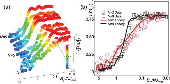
Figure 14. (a) Scaled average absolute magnetization per site, 〈|mS|〉, versus B/NJrms is plotted for N = 2–9 spins. As B/NJrms is lowered, the spin ordering undergoes a crossover from a paramagnetic to FM phase. The crossover curves sharpen as the system size is increased from N = 2 to N = 9, anticipating a QPT in the limit of infinite system size. The oscillations in the data arise due to imperfect initial state preparation and non-adiabaticity due to finite ramping time. (b) Magnetization data for N = 2 spins (circles) are contrasted with N = 9 spins (squares). The data deviate from unity at B/NJrms by ∼20%, predominantly due to spontaneous emissions in Raman transitions and intensity fluctuations of Raman laser beams, as discussed in the text. Here, the theoretical time-evolution curves (red line for N = 2 and black line for N = 9 spins) are calculated by averaging over 10 000 quantum trajectories.
Download figure:
Standard image8. Conclusion and outlook
Trapped atomic ions represent a promising platform for the quantum simulation of intractable Hamiltonian systems. There have been several theoretical proposals in this direction, largely following schemes in the realm of quantum computing, and recent experiments have shown that the system can be scaled to a degree where all classical simulations become impossible [17–19]. This paper has shown both theoretically and experimentally that the quantum simulation of quantum magnetism and the emergence of spin order can be controlled through external laser beams up to nine spins and can further be scaled to much larger numbers of spins. The stable confinement of larger numbers of ions may require novel ion trap architectures such as anharmonic axial potentials [78] for a linear chain or two-dimensional trap geometries [79, 80], but there are no known fundamental limitations in this scaling. As discussed here, for a fixed level of total laser power, the errors associated with decoherence from spontaneous Raman scattering from the lasers is expected to grow only as N1/3 for the linear chain, holding the errors from phonon creation and diabatic transitions to excited states at fixed levels. Alternatively, all these errors can be held at a fixed value independent of N as long as laser power increases by N1/3. In either case the required time for adiabatic ramping grows as N1/3, so slowly drifting errors such as (real) magnetic fields and motional heating of the ions must be kept under control for very large N as discussed in the supplementary information of [17].
This system can also be extended to the Heisenberg or XY Z spin models [12] or spin-1 systems by adding a few more laser beams. As the system grows, the transverse motional modes that mediate the Ising couplings can give rise to higher levels of frustration and complex phases of magnetic ordering. For instance, by preparing the ground state of a highly frustrated collection of trapped ion spins, it should be possible to create localized topological excitations and guide their transport through the system [81]. This example of topological matter is of great interest for the robust representation and manipulation of quantum information [82, 83]. But more generally, the trapped ion system is poised to be the first to determine the ground state features of Hamiltonians where no solution can be obtained otherwise.
Acknowledgments
This work was supported by Army Research Office (ARO) award W911NF0710576 with funds from the DARPA Optical Lattice Emulator (OLE) program, IARPA under the ARO contract, NSF Physics of the Information Frontier Program and the NSF Physics Frontier Center at JQI. JKF also acknowledges support from the McDevitt Endowment Trust of Georgetown University.