
Abstract
Superconducting electric propulsion systems, characterized by high power densities and efficiencies, provide a possibility to zero carbon emission for future aviation. Stacks of high temperature superconducting (HTS) coated conductors (CCs) have become an alternative for high field magnets applied to superconducting machines, given their excellent field trapping ability and thermal stability. High-frequency ripple fields always exist in high-speed electric machines. Most research work regarding HTS trapped field stacks (TFSs) was focused on their magnetization methods and amplitude of trapped flux density; however, their performance in the high-frequency environment remains unclear. Despite several numerical models established for flat HTS TFSs, a comprehensive analysis of curved ones is still lacking, which possess geometrical applicability for cylindrical rotating shafts. Aimed at exploring the electromagnetic properties of curved HTS TFSs applied to high-speed rotating machines, a 3D numerical model considering both the multilayer structure and the Jc(B) dependence of HTS CCs has been built. Current and magnetic flux density distributions, as well as loss properties of a curved HTS TFS have been studied in detail, under perpendicular and cross fields with varying frequencies ranging from 50 Hz to 20 kHz. Results have shown that, the widely adopted two-dimensional-axisymmetric models are inapplicable to study the electromagnetic distributions of TFSs because of the emergence of the electromagnetic criss-cross defined in this paper. High-frequency ripple fields can drive induced current towards the periphery of the HTS TFS due to the skin effect, leading to a fast rise of AC loss and even an irreversible demagnetization of the stack. This paper has qualified and quantified the high-frequency electromagnetic behaviours of curved HTS TFSs, providing a useful reference for their loss controlling and anti-demagnetization design in high-speed propulsion machines.
Export citation and abstract BibTeX RIS

Original content from this work may be used under the terms of the Creative Commons Attribution 4.0 license. Any further distribution of this work must maintain attribution to the author(s) and the title of the work, journal citation and DOI.
1. Introduction
Emissions from aircraft, composed of carbon dioxide, nitrogen dioxide, and sulphates, etc, are causing dramatic air pollution with increasing long-distance international travel [1, 2]. Electric aircraft has been considered as a solution to zero-emission air travel, which requires low weight, high efficiency, and high power density [3, 4]. Superconducting machines, acting as a key component of the electric propulsion system, have provided a possibility for future electric aviation and aerospace industries [5]. The high field source in superconducting machines can be superconducting coils and super permanent magnets. However, aerospace machines need to operate at very high speeds (7–50 kRPM), thus no active windings on the rotor seem to be an ideal choice to reduce the influence of the significant centrifugal stress [6, 7]. Besides, using superconducting coils as field sources generally requires a high current power supply, and they are likely to encounter a sudden failure through quench [8].
Super permanent magnets are composed of bulk superconductors and trapped field stacks (TFSs). High temperature superconducting (HTS) bulks have shown great flux trapping capacity, achieving a world record of 17.6 T at 26 K [9]. However, a crucial problem with HTS bulks is their thermal instability at low temperatures, which makes it difficult to take advantage of the high critical current below 30 K [10]. Besides, external mechanical reinforcement is needed in the application of bulks due to their imperfect mechanical strength. As a comparison, HTS TFSs made of coated conductors (CCs) have better thermal stability, because the silver overlayer and copper stabilizers in HTS CCs have a thermal conductivity over an order of magnitude higher than (RE)BCO. Additionally, as far as mechanical strength is concerned, the Hastelloy substrate in HTS CC has a stronger tensile strength compared to (RE)BCO, thus they can support higher magnetic stresses [10].
Electromagnetic simulation of HTS TFSs is necessary to estimate their field-trapped capacity before the production. Most of the existing numerical models regarding magnetization of HTS stacks are two-dimensional (2D), and the flat stack is modelled as an anisotropic bulk (square or round) in many cases to save computational time [11–14]. For example, in Baskys et al [14] a 2D-axisymmetric model has been employed given that the field trapped in square and round stacks differs by less than 4%. However, we have to note that the magnetic flux density and current density distributions in the round and rectangular tapes are different [15], and 3D modelling is inevitable for a curved spatial geometry [16]. Besides, a comprehensive analysis of curved HTS TFSs is still lacking, which possess geometrical applicability for cylindrical rotating shafts. In many applications, it is sufficient to know the maximum possible trapped field, thus the critical state model assumption can be applied to the simulation of stacks [17]. To achieve the highest trapped field, pulsed filed magnetization (PFM) has been proposed [18–20]. Nevertheless, the magnetization methods and trapped field amplitude are not the focus of this paper. In this study, we aim to investigate the electromagnetic distribution properties of curved HTS TFSs, and it is necessary to consider the field dependence of critical current and model the complete dynamic magnetization process.
Exposed to alternating cross fields, HTS stacks experience a decrease of the trapped field [21–24], and thus a possible demagnetization can happen in a certain situation. The demagnetization of field-trapped magnets would be disastrous for aircraft propulsion and generation systems. In high-speed (7–50 kRPM) rotating machines for future aviation, high-frequency AC ripple fields always exist within the range of ∼0.2–2 kHz [6], and the fields transverse to the surface of CC are abundant. For now, the electromagnetic behaviour of HTS TFSs under high-frequency fields remains unclear. In addition, according to our previous research work [25–28], at frequencies higher than 100 Hz, it is necessary to consider the multilayer physical structure of HTS CCs to quantify magnetization loss due to the skin effect. The existence of the copper stabilizers, silver overlayer, and substrate can influence the loss distribution inside CCs [29]. Page et al [30] has studied the effect of stabilizers on trapped fields of TFSs magnetized by PFM, and demonstrated that the trapped field is insensitive to the stabilizer thickness. However, the influence of high-frequency cross fields on HTS TFSs considering the multilayer structure of each CC is still unknown, i.e. a corresponding 3D numerical modelling work is still lacking.
This paper is a flow-up work of Zhang et al [28], in which we have built an H -formulation based 3D multilayer numerical model for HTS racetrack coils, and validated it with published experimental data. In response to the above-mentioned issues, here we adapt the 3D numerical model in Zhang et al [28] to a curved HTS TFS. Firstly, we have studied the electromagnetic characteristics of a single curved square CC under perpendicular field magnetization. Then, its electromagnetic performance in the time domain during PFM has been presented. Next, under the influence of high-frequency cross fields varying from 50 Hz to 20 kHz, the current and magnetic flux density distributions as well as loss properties of the curved CC after PFM have been investigated. In the end, a case study has been conducted on an HTS TFS composed of five CCs within the same frequency range. This research work is believed to add upon the existing knowledge of HTS TFSs, providing a useful reference for their design and application in high-speed rotating machines for future aviation.
2. Modelling method
The H -formulation based 3D numerical modelling method presented in Zhang et al [28] has been adopted here. The studied HTS CC sample was originally a square tape with a side length of 12 mm, which has been bent into a curved surface with a central angle of 1.2 rad, as shown in figure 1. The sample is a cold-rolled Hastelloy C276 tape, with the functional layers deposited by the IBAD-MgO/PLD-GdBCO route [30]. It is composed of five layers, namely two copper stabilizers with the thickness of 20 μm for each one, a 2 μm-thick silver overlayer, a 1 μm-thick GdBCO layer as well as a 60 μm-thick substrate.

Figure 1. Cross section of the multilayer structure of the studied curved HTS CC, manufactured by SuperOX. (The thickness of each layer does not reflect the real scale.) x, y, and z stand for the axes of the 3D Cartesian coordinate system.
Download figure:
Standard image High-resolution imageAccording to Faraday's law
the constitutive equation

Ohm's law

and Ampère's circuital law

we can obtain the mathematical form of H -formulation, as
where σ and µ represent the conductivity and the permeability of the studied material, respectively, and H stands for the magnetic field intensity.
For the superconducting layer, we have the E–J power law [31]
where E0 denotes a constant with E0= 10−4 V m−1, n is the power index, and Jc( B ) refers to the field-dependent critical current, defined by [32]
where Jc0 is the self-field critical current density, B ⊥ and B ∥ stand for separately the local magnetic flux density perpendicular and parallel to the curved wide surface of the CC. k, α, and B0 are all material-dependent constants, with k = 2.05, and α = 0.65.
H -formulation can be implemented into COMSOL Multiphysics and solved by the finite element method (FEM). The 3D multilayer FEM numerical model of the whole curved square CC is shown in figure 2. The curved CC is surrounded by air, and the Dirichlet boundary condition has been exploited on its outer surface to apply the perpendicular and cross fields.
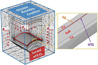
Figure 2. Meshing view of the curved multilayer HTS CC and surrounded air in COMSOL Multiphysics. B e⊥ is the externally applied perpendicular magnetic field, B e ∥1 and B e ∥2 represent the externally applied cross fields.
Download figure:
Standard image High-resolution imageThe specifications and parameter values for simulation of the studied CC sample are summarized in table 1.
Table 1. Specification of the modelled square HTS CC [30].
| Symbols | Quantity | Value |
|---|---|---|
| w | CC side length | 12 mm |
| hHTS | HTS film thickness | 1 μm |
| hCu | Single stabilizer thickness | 20 μm |
| hAg | Silver thickness | 2 μm |
| hsub | Substrate thickness | 60 μm |
| T | Single CC thickness | 103 μm |
| σCu | Copper conductivity at 77 K | 5.076 × 10⁸ S m−1 |
| σAg | Silver conductivity at 77 K | 3.704 × 10⁸ S m−1 |
| σsub | Substrate conductivity at 77 K | 8 × 10⁵ S m−1 |
| μ0 | Free space permeability | 4π × 10–7 H m−1 |
| n | Power-law exponent | 21 |
| Ic0 | Self-field critical current at 77 K | 100 A |
| E0 | Characteristic E-field | 10–4 V m−1 |
| B0 | Magnetic field constant | 1.3 T |
It should be noted that, for the magnetization due to perpendicular magnetic fields, we can model one-quarter of the whole geometry to reduce the numbers of the degree of freedom and save computational time, as presented in Zou [16]. However, once considering the application of cross fields with arbitrary orientation, the boundary condition on the symmetry plane of the quarter model can not be simply determined by the zero flux or Dirichlet boundary condition. Therefore, to apply simultaneously perpendicular and parallel magnetic fields with arbitrary orientations, we have chosen to model the whole geometry at the sacrifice of computational time. It needs to be clarified that here the perpendicular and parallel fields are defined in terms of the 3D Cartesian coordinate system rather than the curved surface, so that a field with arbitrary orientation can always be decomposed into different components along three axes. As shown in figures 1 and 2, Be⊥ refers to the externally applied perpendicular magnetic field, which is along the symmetry line between the x-axis and y-axis. Be ∥1 and Be ∥2 represent the parallel external magnetic fields, which are parallel and perpendicular to the z-axis, respectively.
In order to validate the proposed 3D numerical modelling method, we have built firstly a 3D model for the flat cubic bulk superconductor employed in Benchmark #5 in HTS Modelling Workgroup [33], and then compared the modelling results with the benchmark solutions. More details can be found in appendix.
3. Electromagnetic properties of a single curved CC
In this section, we have simulated the magnetization process of a single curved square HTS CC under AC perpendicular magnetic fields and a pulsed field, respectively. Cross fields of distinct frequencies have been applied to the trapped field CC, and the multilayer electromagnetic distributions have been explored.
3.1. Magnetization by AC perpendicular fields
In this section, the applied perpendicular magnetic field is determined by
Be⊥
= Bext•sin(2πft) + Bext•sin(2πft)
 . Bext is set as 100 mT, and the frequency of the applied field, f, varies from 50 Hz to 20 kHz.
Figure 3 demonstrates the magnetic flux density ((a)–(d)) and current density ((e)–(h)) distributions in the curved square HTS layer at the phase of 3π/2. Although a benchmark model for 3D simulation of a curved square multilayer HTS CC is lacking, the J/Jc distributions in the HTS layer at low frequencies, e.g. at 50 Hz presented in (e), are still comparable to those of the benchmarked flat superconductor in [33]. In (e)–(h), the black arrows describe the current flow direction along the current streamlines, which complies well with Lenz's law. The current streamlines exhibit a rectangular shape and they bend sharply in the 'discontinuity lines' with a lower current density, which coincides with the zero vortex velocity passing through the four corners. More related explanations can be found in Brandt, Badia-Majos and Lopez [15, 34, 35]. Here, we define the 'discontinuity lines' as electromagnetic criss-cross, which divides the curved square surface into four roughly equivalent subdomains.

Figure 3. Magnetic flux density and current density distribution in the curved HTS layer. Bext = 100 mT, and f varies from 50 Hz to 20 kHz. (a)–(d) Represent the magnetic flux density distribution at the phase of 3π/2 for f = 50 Hz, 1 kHz, 10 kHz, and 20 kHz, respectively. (e)–(h) Show separately J/Jc at the phase of 2π for f = 50 Hz, 1 kHz, 10 kHz, and 20 kHz. The black arrows illustrate the current flow direction along with the current streamlines.
Download figure:
Standard image High-resolution imageAccording to figures 3(a)–(d), it can be found that the penetrated magnetic flux will be driven towards the four sides with increasing frequencies, and their amplitudes augment accordingly in a positive way. The same trend also occurs to the current density distribution, i.e. the maximum current density increases positively with frequency and the induced current is pushed to the four sides of the CC.
Nevertheless, it is interesting to note that at higher frequencies in (g) and (h), different from (e) and (f), the current flow direction in the central section is opposite to that in the regions near the edges of the CC. In fact, as shown in (a)–(d), the magnetic flux penetrates into the CC starting from the middle edges, thus the change of current flow directions happens from outside to inside. At low frequencies, after one complete AC cycle, the overturn of current flow directions can be finished. However, at high frequencies, it becomes harder for the magnetic flux to penetrate into the central region due to the skin effect, as shown in (c) and (d). As a result, the induced current in the central part demonstrates a kind of 'lag effect' and seems less sensitive to the variation of external magnetic fields.
The loss per unit volume distributions at the phase of 2π in different layers, defined by E•J (W m−3), have been presented in figure 4. Figures 4(a)–(d) show the loss density distributions in the HTS layer at 50 Hz, 1 kHz, 10 kHz, and 20 kHz, respectively. In the same way, (e)–(h), (i)–(l), (m)–(p) correspond separately to the loss properties in the silver overlayer, substrate, as well as upper copper layer. It is easily understood that, the highest loss density within the frequency range 50 Hz–20 kHz is always generated in the HTS layer because it has the highest electrical conductivity compared to other layers, thus most induced current is concentrated in the HTS layer. Similarly, the loss density in the copper stabilizer is comparable to that of the silver overlayer, both of which are much higher than the loss density in the substrate. For each layer, the power dissipation tends to gather at the CC edges with increasing frequencies, under the skin effect [25, 28]. Consequently, the maximum loss density in every layer grows positively with increasing frequencies.

Figure 4. Distribution of loss per unit volume in different layers. Bext = 100 mT, and f varies from 50 Hz to 20 kHz. (a)–(d) Represent the loss distribution of the HTS layer at the phase of 2π for f = 50 Hz, 1 kHz, 10 kHz, and 20 kHz, respectively. In the same way, (e)–(h) show separately the loss distribution for the silver overlayer, (i)–(l) stand for the loss distribution of the substrate, and (m)–(p) refer to the loss distribution in the upper copper layer.
Download figure:
Standard image High-resolution imageIt can also be found that, for every layer, most of the loss is concentrated on the middle edges of the CC, which cannot be predicted by 2D modelling methods, especially the 2D-axisymmetric model. Evidently, the loss density distribution is determined by both the electric field and current density distributions. Brandt has systematically studied the electric field in superconductors with rectangular cross sections and concluded that, in the critical state flux penetrates mainly from the middle of the edges of the rectangular rather than from the corners [15]. As a result, the varying E•J due to the penetrated magnetic field will be generated starting from the middle edges. At low frequencies, e.g. 50 Hz, figures 3(a) and (e), as well as figure 4(a), comply well with the magnetic field, current, and electric field profiles in Brandt [15].
It is interesting to note that the E•J distribution pattern in the substrate at 50 Hz is peculiar, as shown in figure 4(i), not only different from other layers at the same frequency but also different from the same layer at higher frequencies. It appears that in the vertical and horizontal regions of (i), the power dissipation per unit volume is much lower. In fact, this phenomenon is tightly related to the curvature of the CC. Given that the studied CC is curved and the applied magnetic field, B e⊥ , is perpendicular to the z-axis, B e⊥ is thus not strictly perpendicular to the wide surface of the CC everywhere. In other words, there exist some local parallel field components in the curved CC surface. Under the time-varying local parallel magnetic fields, an eddy current will be induced across the five layers of the CC. Considering that the conductivity of the substrate is much lower than the other layers, and the substrate belongs to the middle layers of the multilayer structure, the eddy current passes through the substrate but does not gather here. As a result, the eddy current will strengthen the current density in the regions located on the current loop, scilicet in these regions, E•J gets higher compared with the vertical and horizontal regions in (i). Figure 5(a) shows the current streamlines on the cross section of the CC in the xy-plane at 50 Hz. In order to better reflect the current density distribution in different layers, the current density has been interpreted by the log transformation with a logarithm base of 10. It can be seen that in the higher E•J regions there exist eddy currents passing through the substrate, rather than in the middle part (lower E•J region), which agrees well with the above analyses. In the two higher E•J regions, the current loop directions are distinct because the local parallel field vectors are different. However, as the frequency increases, the eddy current loops will be driven towards both ends of the CC cross section, i.e. the area in the substrate through which the induced current passes will be reduced. Figure 5(b) demonstrates the current streamlines on the cross section of the CC in the xy-plane at 20 kHz. It can be found that the eddy current generated by the local parallel fields is confined to both ends of the cross section. Besides, the bending angle of the CC is only 1.2 rad, thus the local perpendicular field components are dominant compared to the parallel ones, and this dominance of the local perpendicular fields plays a more significant role at higher frequencies in that the power dissipation increases fast with frequency due to the skin effect. Therefore, at high frequencies, the influence of the local parallel fields on the E•J distribution pattern gets weaken and the penetration effect of the local perpendicular field from the middle edges becomes enhanced.

Figure 5. Logarithmized current density distribution in different layers and current flow arrows on the cross section of the curved HTS CC in the xy-plane at the phase of 2π, under the perpendicular field, B e⊥ . The colour discrepancy represents the current density after the log transformation, and the logarithm base is 10. (a) f = 50 Hz. (b) f = 20 kHz.
Download figure:
Standard image High-resolution imageThe maximum loss density always appears in the HTS layer. However, at high frequencies, when considering the volume of different layers, the majority of loss does not necessarily occur in the HTS layer. The losses produced in distinct layers with varying frequencies have been presented together in figure 6. The loss per unit time (W m−1) in each layer is calculated by
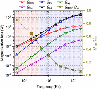
Figure 6. Variation of magnetization losses in different layers, and loss ratio Qdyn/QAC_tot with frequency for the curved square HTS stack. f ranges from 50 Hz to 20 kHz. Bext = 100 mT.
Download figure:
Standard image High-resolution imagewhere V is the total volume of the studied layer.
It can be seen that, from figure 6, generally most of the magnetization loss is concentrated in the HTS layer and copper stabilizers in that they have higher electrical conductivity at 77 K compared to the Hastelloy substrate and silver overlayer. Below 400 Hz, the majority of loss is generated in the HTS layer. However, when the frequency exceeds 400 Hz, the most loss is produced in the copper stabilizers, which is due to the skin effect. The loss ratio between the loss in the HTS layer and the total loss of all the layers, QHTS/Qtot, decreases rapidly from 85% at 50 Hz to approximately 5% at 20 kHz. Therefore, in terms of the quantification of magnetization loss in stacked HTS CCs, it is not accurate to just model the HTS layer, even at power frequencies. On this basis, in the next section, we will investigate the electromagnetic characteristics of the curved square HTS CC magnetized by a typical pulsed field.
3.2. Trapped field CC under cross fields
As mentioned in Zou et al [19, 20], PFM serves as a practical method to magnetize HTS stacks in virtue of its low cost, compactness, and mobility. The frequency band of a pulse is usually abundant, of which the upper cutoff frequency depends closely on its rise time, τ (here rise time refers to the duration in which the pulse amplitude increase from zero to its maxima). We use the single pulse adopted in Zou et al [19] as the applied perpendicular magnetic field, which is defined by
where Bext denotes the maximum amplitude of the pulsed field. Here Bext is set as 2 T, and τ = 10 ms. The time-frequency characteristics of the magnetic field pulse are shown in figure 7, obtained by short-time Fourier transform.

Figure 7. Time-frequency spectrum of the pulsed filed. Bext = 2 T, and τ = 10 ms. STFT: short-time Fourier transform.
Download figure:
Standard image High-resolution imageIt can be seen that, from figure 7, most of the frequency components are concentrated in the band 0–150 Hz, and most of the signal energy is within the time window 0–40 ms.
3.2.1. Perpendicular PFM.
Before applying AC cross fields, we need to investigate the electromagnetic properties of the curved square CC under perpendicular PFM. Given that the primary frequency components of the applied field pulse are within the band of 150 Hz, we just focus on the HTS layer in this section. The magnetic flux density and current density distribution of the curved HTS layer at different time nodes, namely 10 ms, 12 ms, 15 ms, 60 ms, have been presented in figure 8, respectively. (a)–(d) Demonstrate the flux density distribution at the four different time nodes, and (e)–(f) show the J/Jc distribution, accordingly. (a)–(d) Clearly illustrate that the applied field pulse penetrates into the HTS layer from the middle edges of the curved CC, which agrees well with Brandt [15] and the previous analysis. The magnetic flux moves towards the centre and finally, the highest flux density is kept in the central area. The distribution of the trapped flux density also exhibits an electromagnetic criss-cross on the surface of the HTS layer, which cannot be obtained by the conventional 2D modelling methods. (e) and (f) Demonstrate the same trend as (a)–(d), that the induced current gradually occupies all the HTS layer surface from the edges towards the CC centre. It should be underlined that, (f) is actually the intermediate state between (e), the beginning of the current direction change, and (g), the end of the direction change, with the variation of the external pulsed field. Despite the discrepancy of frequencies, figure 8(f) has the same variation characteristics as figures 3(g) and (h), both of which reflect the field trapping routes.

Figure 8. Magnetic flux density and current density distribution in the curved HTS layer under PFM. Bext = 2 T, and τ = 10 ms. (a)–(d) Represent the magnetic flux density distribution at the time nodes of 10 ms, 12 ms, 15 ms, and 60 ms, respectively. (e)–(h) Show separately J/Jc at the time nodes of 10 ms, 12 ms, 15 ms, and 60 ms. The black arrows illustrate the current flow direction along with the current streamlines.
Download figure:
Standard image High-resolution imageOn the basis of section 3.2.1, the influence of cross fields at different frequencies on the trapped field CC will be explored hereinafter. As shown in figure 2, two types of transverse fields, B e ∥1 and B e ∥2 will be separately applied to the CC after PFM, and their amplitude is set as 100 mT.
3.2.2. Cross field parallel to the z-axis.
B e ∥1 is the externally applied cross field parallel to the z-axis. With frequency varying from 50 Hz to 20 kHz, the flux density and current density distribution in the HTS layer at the phase of 2π are presented in figure 9. In general, at frequencies lower than 1 kHz, B e ∥1 does not have a significant influence on the field flux density and current density properties, especially for the trapped magnetic field, compared to figures 8(d) and (h). However, it is interesting that a discrepancy regarding electromagnetic distribution in the direction of the external transverse field appears, which can be found more clearly at high frequencies, as shown in figures 9(c)–(d) and (g)–(h). In fact, at the phase of 2π, the externally applied transverse field is along the negative direction of the z-axis, i.e. from bottom to top as far as the geometrical arrangement of the studied CC in figure 9 is concerned. The electromagnetic criss-cross divides the HTS layer into four parts. Due to the variation of B e ∥1, a current will be induced in the HTS layer, which flows from left to right across the layer surface, named transverse current here. As a result, the current density in the bottom quarter is strengthened, and that in the top quarter part is weakened, as shown in (g) and (h). Accordingly, the current flow direction represented by black arrows in the left and right quarter parts becomes more inclined (not parallel to the edges) under the influence of the transverse current.
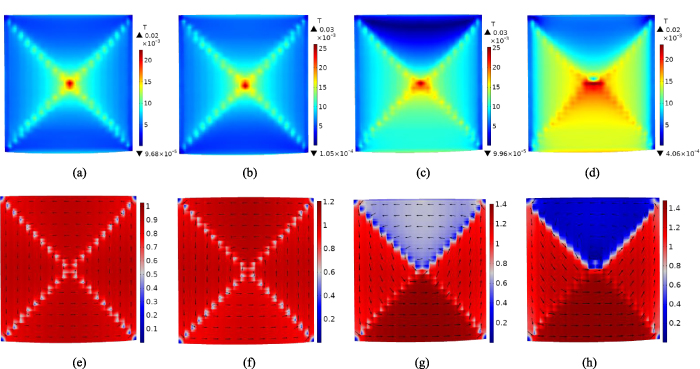
Figure 9. Magnetic flux density and current density distribution in the curved HTS layer. Be∥1= 100 mT, and f varies from 50 Hz to 20 kHz. (a)–(d) Represent the magnetic flux density distribution at the phase of 2π for f = 50 Hz, 1 kHz, 10 kHz, and 20 kHz, respectively. (e)–(h) Show separately J/Jc at the phase of 2π for f = 50 Hz, 1 kHz, 10 kHz, and 20 kHz. The black arrows illustrate the current flow direction along with the current streamlines.
Download figure:
Standard image High-resolution imageTo further illustrate the flowing path of the transverse current, taking f = 20 kHz as an example, the current arrows along the streamlines on the cross sections of the curved CC have been presented in figure 10. Figure 10(a) shows the current density distribution on the cross section in the yx-plane located in the bottom quarter part of figure 9(h), and accordingly (a) demonstrates the current density distribution on the cross section in the xy-plane located in the top quarter region. At the phase of 2π, the applied cross field vector is along the negative direction of the z-axis and the field amplitude is decreasing, thus a counterclockwise current loop has been generated across all the five layers in the yx-plane as shown in (a), which complies well with the Lenz's law. In the same way, a clockwise current loop has been generated in the xy-plane as shown in (b). Taking (a) as an example for detailed analysis, we have enlarged a region of the HTS layer and characterized the amplitude of current density by logarithmic arrow length, as shown in the lower right window (only in the smallest windows of figure 10, the arrow length is logarithmized). It can be seen that the induced current direction due to the cross field coincides with the original current circulating on the wide curved surface, thus the total current has been enhanced, which agrees well with the current variation in the bottom quarter part of figure 9(h). As a comparison, in (b) the induced current direction is opposite to the original circulating current thus the total current has been mitigated in the top quarter section. In addition, according to the colour discrepancies, it can be clearly seen that the current density in the HTS layer of (a) is higher than that of (b). To conclude, the defined transverse current is generated by the externally applied AC cross field, which complies well with Lenz's law.

Figure 10. Logarithmized current density distribution in distinct layers and current flow arrows on the cross sections of the curved CC at the phase of 2π for f = 20 kHz, under the cross field Be∥1 = 100 mT. The colour discrepancy represents the current density after the log transformation, and the logarithm base is 10. (a) Cross section in the yx-plane, located in the bottom quarter part of figure 9(h). (b) Cross section in the xy-plane, located in the top quarter part of figure 9(h).
Download figure:
Standard image High-resolution imageAs for the reason for which this discrepancy appears more obvious at high frequencies, it can be well explained by Faraday's law, in that a higher rate of change of magnetic field leads to a higher induced current, as shown in (1).
3.2.3. Cross field perpendicular to the z-axis.
As the studied square HTS CC has been curved around the z-axis, thus the transverse field perpendicular to the z-axis, B e ∥2, is not parallel to the whole curved surface. Similarly, when the frequency of B e ∥2 varies from 50 Hz to 20 kHz, the flux density and current density distributions in the HTS layer at the phase of 2π are presented in figure 11. Different from the case of B e ∥1, though with the same amplitude, the existence of B e ∥2 has completely changed the electromagnetic distribution of the original trapped field CC, whether at low or high frequencies. In other words, the transverse field B e ∥2 has caused the demagnetization of the original trapped field CC. At frequencies lower than 1 kHz, as shown in (a), (b), (e), and (f), the whole HTS layer can be decomposed into two symmetric curved rectangular CCs, each of which possesses independent magnetization centres and current paths. This phenomenon can be easily explained by Lenz's law, given that B e ∥2 is propagating from right to left when the phase approaches 2π, and its amplitude is simultaneously decreasing. Comparing (a)–(d), it can be found that, with increasing frequency, the penetrated flux is driven towards the left and right edges of the CC under the skin effect. The current streamlines presented in (e)–(h) also show the same trend. However, it is interesting to note that, at frequencies higher than 1 kHz, the streamlines in the central region are no longer parallel to the left or right edge. For example, in (h) the whole HTS layer can be decomposed into three different parts: one current loop in the central section, and two independent current paths near the edges. The current paths on both sides in (h) are similar to those in (e) and (f), though they have been pushed to the left and right edges of the CC under the skin effect. To understand the current loop in the central area, we need to refer to figures 3(g) and (h), because they have the same mechanism. As illustrated before, at high frequencies, the penetrated flux and induced current are constrained near the edges due to the skin effect, thus the current streamlines in the centre tend to remain the same as those of the previous phase. As a result, it becomes harder to change the current path in the central area with increasing frequencies, leading to a 'lag effect'. However, at high frequencies, the current density and magnetic flux density in the central area are much lower than those near the edges, thus this 'lag effect' of electromagnetic distribution does not play a significant role if we only consider where most of the flux and current are concentrated. Nevertheless, it should be underlined that, high-frequency cross fields can easily lead to the demagnetization of the trapped field CC. Therefore, for the design of high-speed superconducting machines equipped with TFSs, the influence of transverse fields, especially B e ∥2, has a significant effect, which must be considered.

Figure 11. Magnetic flux density and current density distribution in the curved HTS layer. Be∥2 = 100 mT, and f varies from 50 Hz to 20 kHz. (a)–(d) Represent the magnetic flux density distribution at the phase of 2π for f = 50 Hz, 1 kHz, 10 kHz, and 20 kHz, respectively. (e)–(h) Show separately J/Jc at the phase of 2π for f = 50 Hz, 1 kHz, 10 kHz, and 20 kHz. The black arrows illustrate the current flow direction along with the current streamlines.
Download figure:
Standard image High-resolution image4. Case study of an HTS stack
In this section, we will model a TFS composed of 5 CCs and study the electromagnetic performance of different layers under cross fields with an arbitrary propagation direction. The applied cross field is the combination of B e ∥1 and B e ∥2, with Be∥1 = 100 mT and Be∥2 = 100 mT.
Before the application of cross fields, the HTS stack is firstly magnetized by the pulsed field adopted in section 3. Figure 12 shows the magnetic flux density distribution in the whole curved stack and the current density distribution in the HTS layers. In figure 8(d), it can be found that the trapped flux in a single curved square CC is concentrated in a small central region. As a comparison, in figure 12(a), the trapped magnetic field in the HTS stack occupies a larger area with a higher flux density, i.e. more flux gets trapped in the stack. Similar to figure 8(h), an electromagnetic criss-cross occurs in figure 12(b) to characterize the current density distribution.

Figure 12. Magnetic flux density and current density distribution in the curved HTS stack after PFM, at 60 ms. Bext = 2 T, and τ = 10 ms. (a) Presents the flux density distribution in the whole stack. (b) Shows the current density distribution in the HTS layers. The black arrows illustrate the current direction along with the current streamlines.
Download figure:
Standard image High-resolution imageTo further describe the trapped field in the stack, the flux density distributions along the z-axis on the upper surface of each CC, namely the top copper surfaces, have been presented in figure 13.

Figure 13. Magnetic flux density distribution along the z-axis on the upper surface of each curved square CC of the HTS stack after PFM, at 60 ms. The CC number is decided from top to bottom.
Download figure:
Standard image High-resolution imageIt can be seen that, from figure 13, the highest trapped flux density appears in the centre of the middle CC (CC 3), which is positioned at the central region of the flux flow traversing the stack. We need to note that, the performance of the TFS is determined by the flux density values in the most top CC, namely CC 1. Although the highest flux density trapped in CC 1 is lower than that of the other CCs, its flux density distribution is more uniform with a smaller variance.
On the basis of the modelling results after one single PFM, the cross fields with different frequencies have been applied. In this section, the cross field is a combination of B e ∥1 and B e ∥2, with Be∥1 = Be∥2 = 100 mT. Figure 14 shows the magnetic flux density in the curved stack at the phase of 3π/2 for f = 50 Hz, 1 kHz, 10 kHz, and 20 kHz, respectively. (a)–(d) refer to the flux density distribution in the upper surface of CC 1. Compared to figure 12(a), it can be seen that, the field distribution under PFM has been changed by the applied transverse fields, i.e. the demagnetization of the TFS has happened. In figure 12(a), most of the trapped flux is concentrated in the central region of the stack. However, in figures 14(a)–(d), the majority of the penetrated magnetic flux appears at the bottom right of the studied surface, along the diagonal (represented by grey dotted lines). In fact, the propagation direction of the synthetic transverse field is approximately along the dotted diagonal, thus it is easy to understand that the highest penetrated flux density appears along the diagonal according to Lenz's law, as shown in (a) and (b). However, at higher frequencies above 1 kHz, the highest flux density emerges on the bottom edges due to the skin effect, as shown in (c) and (d). In other words, the demagnetization of the TFS due to cross fields has become more severe with increasing frequency. To further illustrate the skin effect, the magnetic flux density properties on the diagonal cross section perpendicular to the field propagation direction have been presented in (e)–(h). It can be clearly found that the trapped flux tends to be driven towards the outermost CCs with increasing frequency.

Figure 14. Magnetic flux density distribution in the upper surface of the outermost CC and on the cross section of the curved HTS stack at the phase of 3π/2 under traverse external fields with different frequencies. Be∥1 = Be∥2 = 100 mT. (a)–(d) Represent the flux density distribution in the upper surface of the stack at f = 50 Hz, 1 kHz, 10 kHz, and 20 kHz, respectively. (e)–(f) Stand for separately the flux density distribution on the diagonal cross section of the stack at f = 50 Hz, 1 kHz, 10 kHz, and 20 kHz.
Download figure:
Standard image High-resolution imageFigure 15 shows the magnetization loss in different layers of the curved HTS stack under cross fields with varying frequencies from 50 Hz to 20 kHz. It can be seen that, in general, the losses in different layers are in a positive correlation with the frequency of the external cross fields. When f < 200 Hz, the loss in the HTS layer accounts for more than 90% of the total loss. However, with increasing frequencies, the loss ratio QHTS/Qtot decreases rapidly and attains less than 50% when f exceeds 5 kHz. Therefore, it can be concluded that high-frequency cross fields can lead to high losses in the non-superconducting parts of the HTS stack due to the skin effect. In this case, the multilayer structure of each CC has to be considered in modelling work to accurately predict the electromagnetic performance of the HTS stack under cross fields.

Figure 15. Variation of magnetization losses in different layers, and loss ratio Qdyn/QAC_tot with frequency for the curved square HTS stack under transverse AC fields. f ranges from 50 Hz to 20 kHz. Be∥1 = Be∥2 = 100 mT.
Download figure:
Standard image High-resolution imageIt should be noted that, the field dependence of the critical current of the HTS layer is more sensitive to the perpendicular magnetic fields compared to parallel fields, as shown in equation (7). As a result, under the same frequency and field amplitude, the loss in the HTS layer under cross fields is much lower than that under perpendicular fields. Therefore, in terms of value, the loss of the HTS layer in figure 15 is much lower than that in figure 6, though for the latter there is only one single CC. Besides, magnetization loss increases positively with the surface area exposed to external magnetic fields, which also explains well the fact that the loss values of all the layers in figure 15 are lower than those in figure 6. Due to the same reason, when f > 7 kHz the loss in the substrate exceeds that in the silver overlayer in figure 15, given that the cross-sectional area of the substrate is 30 times larger than that of the silver overlayer, different from the case in figure 6.
5. Discussion
5.1. Temperature dependence
In order to get high trapped flux density, many researchers choose to apply muti-pulse field magnetization techniques to a great number of CCs at very low temperatures, as reported in Baskys et al, Zou et al [18–20]. Nevertheless, targeted at the design of high-speed HTS machines, this paper aims to illustrate the electromagnetic characteristics inside the curved HTS stack under the effect of high-frequency cross fields, rather than study the best magnetization method or to obtain the highest trapped field. Therefore, the magnitude of the trapped field is not a crucial parameter in this study. From this point, here, the temperature has been chosen as 77 K, and a stack composed of only five CCs after one single PFM process has been studied
To model the magnetization of bulk superconductors, normally the temperature dependence of critical current density needs to be taken into account. However, as mentioned in Patel et al [10], TFSs have better thermal stability compared to bulks in that the silver overlayer and copper stabilizers have a much higher thermal conductivity. Therefore, given that the studied stack is not composed of numerous CCs and only one cycle of fields has been applied, in this paper, we assume that the power dissipation can be removed instantaneously, and thus the temperature can be approximated as a constant, 77 K. To verify this assumption, considering the Jc(B,T) dependence, we have modelled the magnetization of a single curved square CC under the AC perpendicular fields used in section 3.1, based on the simulation method presented in Ma et al, Lacroix and Sirois [29, 36]. The Heat Transfer in Solids physics module has been coupled to the H -formulation, with a boundary heat transfer coefficient of 400 W/(m2•K). All the parameters regarding thermal conductivity, heat capacity, and mass density of different materials have been taken from Lacroix and Sirois [36]. Taking f = 50 Hz as an example, the temperature distribution in the HTS layer after one AC cycle is shown in figure 16.

Figure 16. Temperature distribution in the HTS layer of the curved HTS CC under AC perpendicular field magnetization. Bext = 100 mT, and f = 50 Hz.
Download figure:
Standard image High-resolution imageIt can be seen that, the generated heat accumulates starting from the middle edges of the CC, which complies well with figure 4(a) and the conclusions drawn before. Most importantly, the temperature is approximately unchanged with a variation of only 0.2 K. Therefore, it is reasonable to approximate the temperature as a constant in this research. However, we have to clarify that, the heat accumulation is dependent on the number of cycles of the applied AC fields. To study the demagnetization of TFSs due to cross fields of a great number of cycles, more information can be found in a recent publication by Pardo [37].
5.2. Magneto-angular anisotropy
The Jc(B) dependence described by equation (7), proposed by Jiang et al [32], is a semi-empirical Kim model with an orthonormal field dependence, which has been validated experimentally and extensively used in the modelling of HTS stacks and coils [38–42]. Coombs and Ruiz et al have also studied the magneto-angular dependence of Jc, and put forward a more general Jc( B, θ) dependence as [43, 44]
with

where θ represents the angle between the field vector and the crystallographic ab-plane of the HTS layer (i.e. when B is perpendicular to the wide surface of the CC, θ= π/2), γ refers to the electron mass anisotropy ratio, α and β are both constants.
Four different material law models have been systematically compared in Robert et al [44], including (7) and (10). It is concluded that when at a low transport current (below 0.4 Ic0), the magnetization losses obtained by (7) and (10) are almost the same. In fact, (7) is in essence a simplified version of (10) with specific parameters. In this paper, the transport current in HTS stacks is zero, thus it is reasonably considered that (7) can reflect well the magneto-angular anisotropy of CCs in terms of loss quantification.
In addition, to avoid ambiguity, it should be clarified here that though the studied HTS stack is curved, the orthonormal field dependence has been well considered. As illustrated in figure 19 in Zhang et al [28], the Jc(B) dependence is closely linked to the angle between the field vector and the wide surface normal of the CC. Then, the local parallel and perpendicular flux densities at the studied point can be expressed as
where Bx and By stand for the flux density components along the x-axis and y-axis, respectively; τ and n represent the unit tangent vector and unit normal vector at any studied point on the curved surface. More information can be found in Zhang et al [28].
6. Conclusion
This paper is a follow-up work of our previous publications [25–28]. TFSs are a potential field source applied to high-speed HTS machines. Based on the proposed 3D numerical modelling method in Zhang et al [28], the electromagnetic characteristics of curved TFSs under the influence of frequency-varying perpendicular and cross fields have been investigated, within the range of 50 Hz–20 kHz. The adopted H -formulation based 3D numerical modelling method has been validated through comparison with Benchmark #5 in terms of a flat cubic bulk superconductor in HTS Modelling Workgroup [33]. The whole modelling work has considered the multilayer physical structure of each HTS CC, namely the HTS and non-superconducting layers.
The electromagnetic characteristics of magnetized HTS stacks, including current density and magnetic flux density distributions, cannot be correctly predicted by the widely adopted 2D-axisymmetric models because of the emergence of the electromagnetic criss-cross. The defined electromagnetic criss-cross in this paper divides the CC wide surface into four roughly equivalent subdomains. Therefore, 3D numerical modelling methods need to be adopted. As for loss properties, the multilayer physical structure of HTS CCs has to be considered, especially for perpendicular field magnetization even at low-frequency band, e.g. at 50 Hz. For cross field magnetization, the multilayer structure has to be taken into account at frequencies higher than 200 Hz.
For perpendicular field magnetization of curved HTS stacks, the applied field starts to penetrate into the stack from the middle edges. As a result, at high frequencies, the skin effect can focus the penetrated flux and induced current due to Lenz's law near the edges. In other words, the induced current in the central part of the curved square CC demonstrates a kind of 'lag effect' in the time domain and seems less sensitive to the variation of external magnetic fields.
Two types of cross fields have been studied. Under the cross field completely parallel to the curved surface, B e ∥1, a transverse current can be generated. The transverse current can enhance the current in one quarter subdomain of the HTS layer and mitigate the current in another quarter section, which agrees well with Lenz's law on the macro level. Under the cross field traversing the curved surface, B e ∥2, the curved surface can be decomposed into two symmetric curved rectangular CCs, each of which possesses independent magnetization centres and current paths. Due to the influence of cross fields on the electromagnetic distributions and loss characteristics, demagnetization can happen to the TFS. With increasing frequencies of cross fields, the originally trapped flux after PFM in the stack can be deteriorated more severely due to the skin effect.
To sum, different from other researchers' work, this paper has not looked into the best magnetization method or highest trapped field in terms of TFSs, but has focused on their dynamic electromagnetic characteristics under high-frequency perpendicular and cross fields. This work further adds upon the existing knowledge regarding TFSs, and is believed to provide a useful reference for their application in high-speed superconducting propulsion machines for future aviation. The proposed 3D numerical model for TFSs can be extended to the study of HTS stacks (flat and curved) without copper stabilizers, or with magnetic substrates.
Acknowledgments
This work was supported by the joint scholarship from the University of Edinburgh and China Scholarship Council (CSC) under Grant [2018] 3101.
: Appendix
Given that a benchmark model for a curved HTS CC or a trapped field stack is still lacking, we have firstly build a 3D flat cubic bulk superconductor model based on H -formulation and compared the simulation results with Benchmark # 5 in HTS Modelling Workgroup [33]. The established numerical model in COMSOL Multiphysics and the bulk dimensions can be found in figure A1. Considering the symmetry of the cubic bulk, to save computational time, we have chosen to model a quarter of it. It should be noted that, the zero flux boundary condition needs to be applied to the symmetrical cross sections because the external magnetic field is along the z-axis. The applied magnetic field is sinusoidal with the amplitude of 200 mT and the frequency of 50 Hz. The critical current density of the bulk superconductor is set as Jc0 = 108 A m−2.

Figure A1. One quarter meshing view of the falt cubic bulk superconductor and surrounded air in COMSOL Multiphysics. B e⊥ is the externally applied perpendicular sinusoidal magnetic field.
Download figure:
Standard image High-resolution imageTaking J/Jc0 at the phase of 2π at the plane z = 0.12 mm as an example, the benchmark solution and the modelled result are both shown in figure A2. Besides, the current density ratio Jz/Jc0 along the x-axis at y = 2.07 mm and z = 1.1 mm is presented in figure A3. The benchmark solutions in figures A2 and A3 are obtained by using the Minimum electro-magnetic entropy production method [33]. It can be seen that the simulation results are in good accordance with the benchmark solutions, thus it is believed that the adopted 3D modelling method in this paper is validated. In the H -formulation based model, we have then replaced the cubic bulk superconductor with the curved HTS CC and stack. Afterwards, the article body has centred around the modelling work of the curved HTS CC and stack.
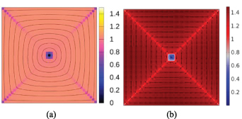
Figure A2. J/Jc0 at the phase of 2π at the plane z = 0.12 mm for the benchmark cubic bulk superconductor model and the model built in this paper. (a) Represents the benchmark solution [33]. (b) Shows the modelled result, in which the black arrows illustrate the current direction along with the current streamlines.
Download figure:
Standard image High-resolution image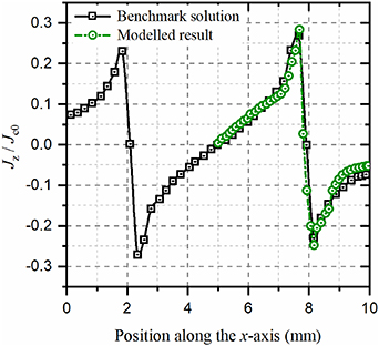
Figure A3. Jz /Jc0 along the x-axis at y = 2.07 mm and z = 1.1 mm for the benchmark cubic bulk superconductor model and the model built in this paper. The benchmark solution is obtained using MEMEP, and the relevant data are extracted from figure 7 in [33].
Download figure:
Standard image High-resolution image