

Abstract
Conventional viscoelastic dampers based on common elastomers cannot adjust their stiffness to adapt to complex vibration conditions. To overcome this shortcoming, a novel stiffness tunable viscoelastic (STV) damper is proposed in this study. Electrorheological elastomers (EREs), which present a tunable storage modulus by applying electric fields, were used as the key materials to provide the STV damper with electric field responsive stiffness. A series of experiments was conducted to study the dynamic mechanical properties of the STV damper under different displacement amplitudes, frequencies, and electric field strengths. The results indicated that the force–displacement hysteretic curve of the STV damper depends on displacement amplitude and frequency, and could be actively controlled by the electric field strength. Consequently, the equivalent stiffness, equivalent damping, equivalent damping ratio, and energy dissipation capacity of the STV damper were electric field responsive terms. A mechanical model of the STV damper was established on the basis of the material constitutive. The simulation results obtained by the model agreed well with the experimental data, indicating that the model can be used for semi-active control of the STV dampers.
Export citation and abstract BibTeX RIS
1. Introduction
Structural vibration control is always an important concern when engineers design structures [1, 2]. Plenty of dampers have been developed to reduce the vibration of structures, such as viscous dampers, metallic dampers, friction dampers, viscoelastic dampers, and so on [3–5]. Viscoelastic dampers have achieved some applications due to their good damping performance [6, 7]. However, just like other passive dampers, viscoelastic dampers are only effective for vibration control in a limited frequency range. The fact is that in most cases, the input vibration is random and in a wider range. As a result, passive dampers could reduce structural vibration in some cases, but fail to reduce the vibration or even increase the vibration under other conditions. Providing viscoelastic dampers with tunable stiffness or tunable damping capacity is a method to solve this problem. Such kinds of dampers could adjust their stiffness or damping to adapt to various vibration conditions. Recently, a few stiffness tunable viscoelastic (STV) dampers have been proposed. Tu et al designed an adjustable stiffness viscoelastic damper using magnetorheological elastomers (MREs). The research suggested that the new damper had continuously adjustable shear stiffness with changing magnetic fields [8]. However, since the stiffness is controlled by the magnetic field, such dampers have shortcomings such as complex design, heavy weight, poor stability, slow response, and thermal disturbance of magnetic circuit [9–14].
Electrorheological elastomer (ERE) is a new smart material with tunable dynamic viscoelasticity, including storage modulus, loss modulus, and damping factor. Typical EREs are prepared by dispersing polarizable particles within an elastomer matrix. Unlike MREs, they are responsive to electric fields rather than magnetic fields. Therefore, the heavy electromagnetic coils that are necessary in MRE devices can be abandoned, which gives devices based on EREs such advantages as simpler design, lower weight, and faster response [15, 16]. By applying an electric field, the electrostatic interaction between adjacent particles makes the stiffness of the elastomers increase, and the higher electric field will lead to higher stiffness [17–19]. By comparison with electrorheological fluids (ERFs), since the carrier liquids are replaced by elastomers, EREs overcome the shortcomings of sedimentation of particles and leakage of fluids [20, 21].
According to the arrangement of dielectric particles in an elastomer matrix, EREs can be classified into isotropic EREs and anisotropic EREs. The particles in anisotropic EREs are aligned by applying an orientation electric field during the curing process, while in isotropic EREs, the particles are randomly distributed. A number of studies have proved that anisotropic EREs present a much more significant electric field induced storage modulus than isotropic elastomers [22–26]. A few scholars have used EREs to reduce structural vibration. For example, in 2013, Zhu et al applied EREs to shear shock absorbers and squeeze shock absorbers, which indicated that the vibration amplitude under an external electric field was smaller than that without an electric field [27, 28].
EREs also have the potential to be used to develop STV dampers. With respect to STV dampers based on MREs, ERE-based STV dampers are expected to overcome the shortcomings mentioned above. Unfortunately, traditional EREs had a low storage modulus and weak electric field response, which cannot be used in practical engineering [29, 30]. In 2015, we used urea-coated TiO2 particles as the dispersing phase to prepare silicone rubber matrix-based EREs [31]. Due to the enhanced polarization by urea coating, the new EREs present a much higher storage modulus and wider storage tunable range than the traditional materials. The development of high-performance EREs allows the design of new STV dampers to become practical. In this study, an STV damper was designed based on the new EREs and tested under various conditions. Its electric responsive dynamic mechanical properties were especially investigated on a hydraulic fatigue machine coupled with a high-voltage DC power supply. Furthermore, a mechanical model composed of a Bouc–Wen model in parallel with a Kelvin solid and an air spring was established. The aim of this study is to develop a new STV damper based on EREs and evaluate its performance. The new STV damper would have such merits as simple structure, short response time, and low weight, and would have a promising future in practical applications.
2. Experiment and results
2.1. Preparation of EREs
TiO2 nanoparticles with a urea coating were used as the dispersing phase to prepare the EREs [31]. The EREs were made using the following procedure. First, silicon RTV-615 was mixed with silicon oil. Then, the particles were introduced into the mixture and mechanically stirred for 30 min. The as-obtained electrorheological mixture contained 35% silicon RTV, 35% silicon oil, and 30% dielectric particles in volume. Subsequently, the catalyst was added to the mixture and vigorously stirred with a motor stirrer for 5 min. To remove the entrapped air, the mixture was transferred into a vacuum case. Then it was filled in the mold before vulcanizing. To align the particles, two electrode plates were inserted into the mold and the rubber mixture was subjected to a constant electric field of 1 kV mm−1 at room temperature during the curing process. The curing time was 24 h.
2.2. Design of construction
The EREs, which were 30 × 30 × 1 mm in size, were then used as the key materials to fabricate an STV damper. The thickness was determined so that the EREs were under 100% strain at 1 mm displacement. The structure of the damper is illustrated in figure 1. In terms of insulation, plexiglass was used to make the two fixed plates of the damper, which were rectangles measuring 180 × 140 × 15 mm. Two small copper plates were glued to the EREs and the fixed plates served as negative electrode plates. The core plate of the damper that was glued to the two pieces of ERE acted as the slider and the positive electrode plate. Subsequently, three fixed steel spacers were applied between the two fixed plates for the purpose of controlling the gap and ensuring the axial movement of the slider. The lower spacer also acted as the fixed end of the damper.
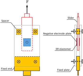
Figure 1. Structure diagram of STV damper based on EREs.
Download figure:
Standard image High-resolution image2.3. Experimental method
A hydraulic fatigue machine was used to test the force–displacement hysteresis curves of the STV damper under different conditions, as shown in figure 2. A high-voltage DC power supply (LSL-60) was used to apply the electric field. The electric field was directly displayed on the power supply; as a result, the electric field strength can be calculated through dividing the electric field by the thickness of the ERE. Table 1 shows the test scheme of the STV damper under sinusoidal excitation. The test conditions were determined according to the Technical Specification for Seismic Energy Dissipation of Buildings of China [32]. The maximum strain amplitude of the ERE was 100%, and the shear frequency was within the range 0.1– 2 Hz. There were two reasons to restrict the frequency below 2 Hz. First, the restriction was a consideration of practical working conditions. Viscoelastic dampers are usually applied to control the vibrations of engineering structures with low natural frequencies, such as high-rise buildings, base isolated buildings and the cables of the cable-stayed bridges. Most of the fundamental natural frequencies of these structures are below 2 Hz. Second, the restriction was a consideration of experimental accuracy. It is known that the inertial force is proportional to the square of the loading frequency. If the loading frequency is high, the inertial force of the experimental system will become significant. As a result, the restoring force measure will become inaccurate.

Figure 2. An image of the experimental system of the STV damper.
Download figure:
Standard image High-resolution imageTable 1. Test scheme of the STV damper.
| Shear displacement amplitude (mm) | Shear frequency (Hz) | Electric field strength (kV mm−1) |
|---|---|---|
| 0.1 | 0.1, 0.5, 1, 2 | 0, 1, 2 |
| 0.2 | 0.1, 0.5, 1, 2 | 0, 1, 2 |
| 0.3 | 0.1, 0.5, 1, 2 | 0, 1, 2 |
| 0.4 | 0.1, 0.5, 1, 2 | 0, 1, 2 |
| 0.5 | 0.1, 0.5, 1, 2 | 0, 1, 2 |
| 0.6 | 0.1, 0.5, 1, 2 | 0, 1, 2 |
| 0.7 | 0.1, 0.5, 1, 2 | 0, 1, 2 |
| 0.8 | 0.1, 0.5, 1, 2 | 0, 1, 2 |
| 0.9 | 0.1, 0.5, 1, 2 | 0, 1, 2 |
| 1.0 | 0.1, 0.5, 1, 2 | 0, 1, 2 |
2.4. Results and discussion
2.4.1. Force–displacement hysteresis curves
Force–displacement hysteresis curves under various conditions were obtained. For a concise overview, several typical results are presented in this study. Figure 3 shows the force–displacement hysteresis curves obtained under constant frequency (1 Hz) and electric field (1 kV mm−1), but various displacement amplitudes. Figure 3(a) shows the hysteresis curves under low displacement amplitude levels (0.1– 0.4 mm), while figure 3(b) shows the data under high displacement amplitude levels (0.5 –1 mm). As shown in figure 3(a), the hysteresis loop under low displacement amplitude presents a fusiform shape. The slope of the main axis of each hysteresis curve, which represents the stiffness of the damper, gradually decreases with increasing strain amplitude. This can be attributed to the decreasing storage modulus of the EREs with increasing strain amplitude at low strain amplitude levels, which is due to the Payne effect. Nevertheless, under high displacement amplitude levels, the shape of the hysteresis loop is not fusiform, and the slope of the main axis increases with increasing displacement amplitude. The phenomenon originated from the strain-hardening of the EREs, which can be attributed to the stretched segments of the molecules of the silicone rubber. Under high shear strain levels, the applying force should overcome the covalent bonds of the silicone rubber, resulting in increasing storage modulus as the strain amplitude rises.
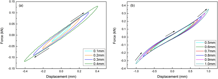
Figure 3. Force–displacement hysteresis curves obtained under constant frequency (1 Hz), constant electric field (1 kV mm−1), and various displacement amplitudes. (a) Small displacement amplitudes, (b) large displacement amplitudes.
Download figure:
Standard image High-resolution imageFigure 4 shows the force–displacement hysteresis curves obtained under constant displacement amplitude (0.5 mm) and electric field (1 kV mm−1), but at various shear frequencies (0.1, 0.5, 1, and 2 Hz). The slope of the main axis of each hysteresis curve as well as the bearing force increase with increasing shear frequency. This can be attributed to the promotion of the storage modulus of the ERE with increasing shear frequency [31]. For example, the bearing force of the damper tested under 0.1 Hz was 144 N, while it was 166 N under 2 Hz.
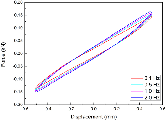
Figure 4. Force–displacement hysteresis curves obtained under constant displacement amplitude (0.5 mm), constant electric field (1 kV mm−1), and various shear frequencies (0.1, 0.5, 1, and 2 Hz).
Download figure:
Standard image High-resolution imageThe dependence of the force–displacement hysteresis curve on the displacement and frequency of the STV damper is similar to conventional viscoelastic dampers. The unique property of the STV damper is the electric-field-dependent dynamic viscoelasticity. Figure 5 shows the hysteresis loops tested under constant shear frequency (0.5 Hz) and constant displacement amplitude (0.7 mm), but different electric field strengths (0 kV mm−1, 1 kV mm−1, 2 kV mm−1). Obviously, the slope of the main axis of the hysteresis loops (the dotted lines) increases with increasing electric field. This is attributed to the positive relationship between the storage modulus of the EREs and the electric field. The results indicate that the stiffness of the STV damper can be actively controlled by applying different electric fields.

Figure 5. Hysteresis loops tested under constant shear frequency (0.5 Hz), constant displacement amplitude (0.7 mm), and different electric field strengths (0 kV mm−1, 1 kV mm−1, 2 kV mm−1). The dotted lines represent the main axis of the hysteresis loops.
Download figure:
Standard image High-resolution imageIt should be pointed out that although the relative change of the storage modulus of the EREs was significant in material tests carried out by the rotary rheometers [31], the relative change of the stiffness of the STV damper is relatively smaller. The reason is that the ERE layers show a hardening nonlinear stiffness because of tension, causing the general stiffness to increase significantly. As a result, the relative stiffness change caused by the electrorheological effect becomes less remarkable due to the significant general stiffness increase. Although the observed stiffness change is small, the STV damper still has its applications due to its continuous and real-time tunable stiffness. For example, the STV dampers can be made into variable-stiffness tuned mass dampers (TMDs). In such applications, when the natural frequency of the TMD is tuned to the natural frequency of the main structure, the structural response can be significantly controlled. Moreover, the control performance of TMDs is very sensitive to the frequency ratio. A frequency error of 2% could double the structural response. As the natural frequency of the engineering structure may slightly change for a couple of reasons (temperature change, structural damage, construction error, corrosion, etc), the STV damper can be applied to retune the TMD system, ensuring the best performance of vibration control.
2.4.2. Equivalent stiffness, equivalent damping, and equivalent damping ratio
Based on the hysteresis curves obtained under different conditions, the equivalent stiffness k', equivalent damping c', and equivalent damping ratio ξ of the STV damper were calculated according to Soong's theory [33], as follows,
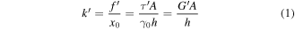


where f' and f'' are the damping force at the maximum displacement and at zero displacement, respectively. x0 and γ0 are the maximum displacement and the maximum shear strain, respectively. τ' and τ'' are the shear stress at the maximum displacement and at zero displacement, respectively. A and h are the shear area and thickness of the ERE, respectively. G' and G'' are the storage modulus and loss modulus of the ERE, respectively. ω is the excitation frequency. Table S1 is available online at stacks.iop.org/SMS/29/045041/mmedia and lists the equivalent stiffness of the STV damper under different conditions.
To find the detailed influence of the displacement amplitude, shear frequency, and electric field on the equivalent stiffness of the STV damper, surface diagrams under constant frequency (0.1 Hz), constant displacement (0.3 mm), and constant electric field (1 kV mm−1) are presented in figure 6. These indicate that the equivalent stiffness of the STV damper increases with increasing electric field and frequency. However, the relationship between the equivalent stiffness of the damper and displacement amplitude is not monotonous; initially, it decreases with increasing displacement amplitude at low levels, and then increases with increasing displacement amplitude. The decreasing equivalent stiffness at low displacement levels was attributed the Payne effect of the ERE, while the promotion at high displacement amplitude levels was caused by the strain-hardening of the ERE. These results agree with figure 3.
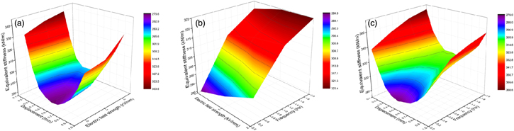
Figure 6. Equivalent stiffness of STV damper under (a) 0.1 Hz, (b) 0.3 mm, and (c) 1 kV mm−1.
Download figure:
Standard image High-resolution imageTable S2 lists the equivalent damping of the STV damper under different conditions. To find the detailed influence of the displacement amplitude, shear frequency, and electric field on the equivalent damping of the STV damper, surface diagrams under constant frequency (0.1 Hz), constant displacement (0.3 mm), and constant electric field (1 kV mm−1) are presented in figure 7. These indicate that the equivalent damping of the STV damper increases with increasing displacement amplitude or decreasing shear frequency. In particular, the electric field has a positive influence on the equivalent damping of the STV damper, which is consistent with the fact that the loss modulus of the EREs increases with increasing electric field [31].
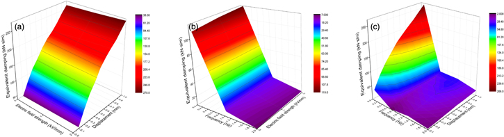
Figure 7. Equivalent damping of STV damper under (a) 0.1 Hz, (b) 0.3 mm, and (c) 1 kV mm−1.
Download figure:
Standard image High-resolution imageThe equivalent damping ratio is another important parameter to evaluate the viscoelastic dampers. Table S3 lists the equivalent damping ratio of the STV damper under different conditions. To find the detailed influence of the displacement amplitude, shear frequency, and electric field on the equivalent damping of the STV damper, surface diagrams under constant frequency (0.1 Hz), constant displacement (0.3 mm), and constant electric field (1 kV mm−1) are presented in figure 8. These indicate that the equivalent damping ratio of the STV damper dramatically increases with increasing displacement amplitude, and slightly rises with increasing shear frequency. However, the relationship between the equivalent damping ratio and the electric field is complex. Since both G' and G'' are electric field dependency parameters, the ratio between them varies with electric field, and is a nonlinear function of the electric field.
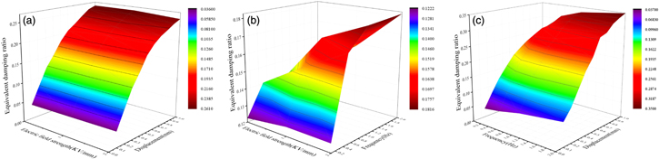
Figure 8. Equivalent damping ratio of STV damper under (a) 0.1 Hz, (b) 0.3 mm, and (c) 1 kV mm−1.
Download figure:
Standard image High-resolution image2.4.3. Energy dissipation capacity
As a damper, the STV damper can dissipate the input energy. The energy dissipation capacity can be quantitatively evaluated by calculating the envelope area of each force–displacement curve. The specific data are listed in table S4. Figure 9 shows the dependence of the energy dissipation capacity of the STV damper on the displacement amplitude. As the displacement amplitude increases, the energy dissipation capacity of the STV damper significantly increases. It can also be seen that the energy dissipation capacity under the higher electric field is higher than under lower field strength.
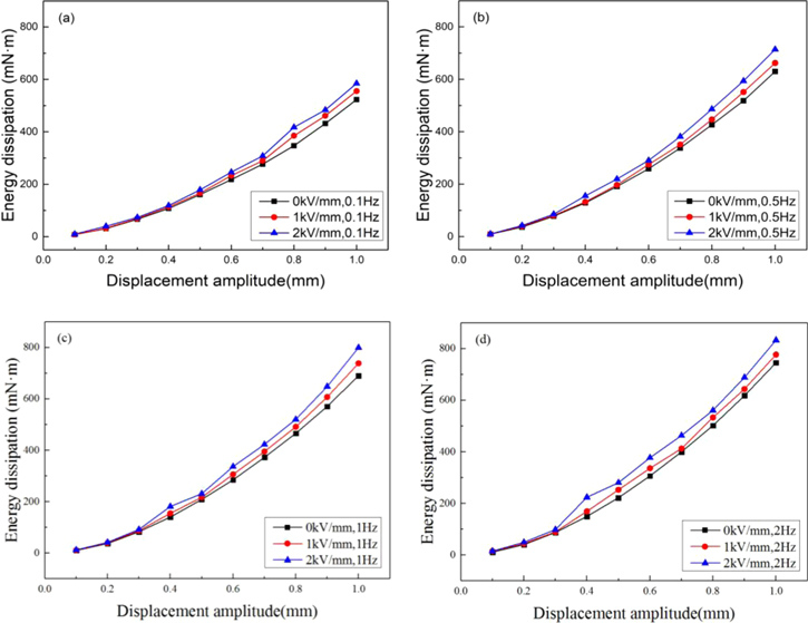
Figure 9. Dependence of energy dissipation on displacement amplitude under different shear frequencies. (a) 0.1 Hz, (b) 0.5 Hz, (c) 1 Hz, and (d) 2 Hz.
Download figure:
Standard image High-resolution imageFigure 10 shows the dependence of the energy dissipation capacity of the STV damper on the shear frequency under constant electric field (1 kV mm−1) but different displacement amplitudes. The energy dissipation capacity of the STV damper positively depends on the shear frequency. Such a dependence is more significant under larger displacement amplitudes.
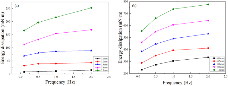
Figure 10. Dependence of energy dissipation on shear frequency under constant electric field (1 kV mm−1) and different displacement amplitudes. (a) Small displacement amplitude (0.1–0.5 mm), and (b) large displacement amplitudes (0.6–1.0 mm).
Download figure:
Standard image High-resolution imageAll of the above results, the positive relationship between the energy dissipation capacity and the displacement amplitude or frequency, are similar to those of passive viscoelastic dampers. The difference between the STV damper and conventional viscoelastic dampers is its electric-field-dependent energy dissipation capacity, as shown in figure 11. As the electric field rises, the energy dissipation capacity of the STV damper increases. Such an electric-field-dependent energy dissipation capacity is weak at low displacement amplitude levels, but is significant at high displacement amplitude levels. This indicates that we can tune the energy dissipation capacity of the STV damper by applying different electric fields.
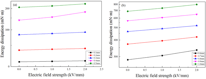
Figure 11. Dependence of energy dissipation on electric field strength under constant frequency (0.1 Hz) and different displacement amplitudes. (a) Small displacement amplitude (0.1–0.5 mm), and (b) large displacement amplitudes (0.6–1.0 mm).
Download figure:
Standard image High-resolution image3. Mechanical model
A mechanical model is established to simulate the performance of the STV damper.
The model consists of a Bouc–Wen model in parallel with a Kelvin solid and an air spring, as shown in figure 12. The Bouc–Wen model and the spring in the Kelvin solid are used to simulate the nonlinear dependence and linear dependence of force on displacement, respectively, while the dashpot in the Kelvin solid is mainly used to describe the relationship between force and velocity. The air spring element is used to reflect the strain-hardening phenomenon of the hysteretic curve. Therefore, the force is given by

where F and  are the force and displacement amplitude, respectively.
  and
and  are the stiffness of the spring in the Kelvin solid and air spring, respectively.
  is the viscosity coefficient of the Kelvin solid. A, n,
  , and
, and  are coefficients that influence the shape and size of the hysteresis loops.
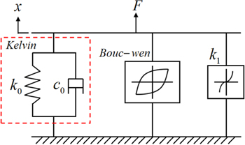
Figure 12. Mechanical model of the STV damper.
Download figure:
Standard image High-resolution imageFigure 13 shows the experimental and simulated data under the loading cases of 0.5 Hz frequency, 0.8 mm displacement amplitude, and 1 kV mm−1 electric field strength. Since n has little influence on hysteresis loops, n = 1 is predetermined for simplification. The other parameters are identified as  = 0.075 N mm−1,
  = 0.236 N mm−3, A = 0.13,
  = 13,
= 13,  = −6.5, and
  = 0.005 Pa · s. The simulation results accurately describe a force–displacement curve, a force–velocity curve and a force–time curve.
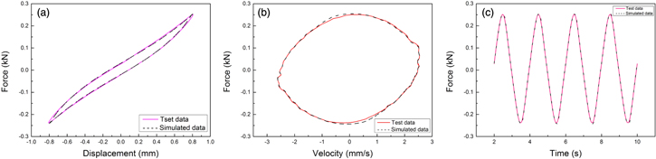
Figure 13. Experimental and simulated data under the loading cases of 0.5 Hz frequency, 0.8 mm displacement amplitude, and 1 kV mm−1 electric field strength. (a) Force versus displacement, (b) force versus rate, and (c) force versus time.
Download figure:
Standard image High-resolution imageTo further validate the accuracy of the mechanical model, the simulated force–displacement curves under various loading cases are obtained and compared with the experimental data, as shown in figure 14. The results indicate that the simulated force–displacement curves obtained by the model agree well with the experimental data.

Figure 14. Comparisons between the experimental hysteresis loops and simulated results of the STV damper under various conditions.
Download figure:
Standard image High-resolution image
To evaluate the accuracy of the restoring force model, the fitting precision R2 values under those loading conditions were calculated, as listed in table S5. For all of the loading conditions, R2 values were larger than 0.99. This indicated that the simulated results obtained by the model agree well with the experimental data. Therefore, the established mechanical model could describe and predict the performance of the STV damper under low frequency (0.1–2 Hz), shear displacement amplitudes from 0.1 mm to 1 mm and electric field intensity from 0 kV mm−1 to 2 kV mm−1.
The parameters of the mechanical model are shown in table 2. The A, β, and γ of Bouc–Wen are constant parameters in the specified working condition and do not change with field intensity and shear frequency. It is true that the other parameters vary with loading frequencies and electric field. Meanwhile, in figures 14(a)–(i), it is also proven that the parameters are independent from the deformation amplitudes. As the parameters vary with electric field, the electrorheological effect can be quantified by the variation of these parameters. For engineering structures, the oscillation amplitude will increase dramatically when the dominant loading frequencies are close to their natural frequencies, known as resonance. To control such resonant vibrations, SVT dampers can be used. In resonant vibration cases, the loading frequencies do not change that much, while the loading amplitudes may vary. As a result, the model with frequency-dependent and amplitude-independent parameters is acceptable to simulate the device's responses.
Table 2. Identified parameters of the mechanical model.
| Field intensity (kV mm−1) | Frequency (Hz) | k0 (N mm−1) | k1 (N mm−3) | A | β | γ | n | c0 (Pa · s) |
|---|---|---|---|---|---|---|---|---|
| 0 | 0.1 | 0.051 | 0.233 | 0.13 | 13 | −6.5 | 1 | 0.01 |
| 0.5 | 0.07 | 0.236 | 0.13 | 13 | −6.5 | 1 | 0.005 | |
| 1 | 0.075 | 0.237 | 0.13 | 13 | −6.5 | 1 | 0.0033 | |
| 2 | 0.076 | 0.238 | 0.13 | 13 | −6.5 | 1 | 0.0015 | |
| 1 | 0.1 | 0.056 | 0.234 | 0.13 | 13 | −6.5 | 1 | 0.01 |
| 0.5 | 0.075 | 0.236 | 0.13 | 13 | −6.5 | 1 | 0.005 | |
| 1 | 0.08 | 0.237 | 0.13 | 13 | −6.5 | 1 | 0.0033 | |
| 2 | 0.083 | 0.245 | 0.13 | 13 | −6.5 | 1 | 0.0015 | |
| 2 | 0.1 | 0.068 | 0.235 | 0.13 | 13 | −6.5 | 1 | 0.01 |
| 0.5 | 0.078 | 0.243 | 0.13 | 13 | −6.5 | 1 | 0.005 | |
| 1 | 0.081 | 0.245 | 0.13 | 13 | −6.5 | 1 | 0.0033 | |
| 2 | 0.084 | 0.25 | 0.13 | 13 | −6.5 | 1 | 0.0015 |
4. Conclusion
To provide viscoelastic dampers with tunable performance for better vibration control, a novel STV damper was fabricated based on EREs, which present tunable dynamic viscoelasticity under different electric fields. The tests results indicated that the force–displacement hysteretic curve of the STV damper can be actively tuned by applying electric fields. Its equivalent stiffness, equivalent damping, equivalent damping ratio, and energy dissipation capacity vary with electric fields as well as the displacement amplitudes and frequencies. As the electric field increases, its equivalent stiffness, equivalent damping, and energy dissipation capacity increase. Therefore, the STV damper has the potential to be used to control the vibration of structures in complex conditions by tuning the electric field. Furthermore, a mechanical model composed with a Bouc–Wen model in parallel with a Kelvin solid and an air spring was established. This could simulate and predict the force–displacement hysteretic curves of the STV damper under various conditions, and was acceptable to simulate the damper's responses for semi-active control.
Acknowledgments
This research is funded by the National Key R&D Program of China under Grant Number 2018YFC0705603 and the National Natural Science Foundation of China under Grant Number 51478088.