

Abstract
Delamination is one of the common damages affecting the safety of composite structures. In this paper, a Lamb wavefield-based monogenic signal processing algorithm is proposed to quantify the delamination parameters in composite laminates, including location, size, shape, and depth. A quality-guided fast phase unwrapping algorithm is developed to solve the problem of phase wrapping after Riesz transform-based monogenic signal processing. Then, space distribution of the phase of Lamb wavefield can be extracted for calculating wavenumber distribution, which is related to the structural thickness or delamination depth and can be used for delamination imaging. Simulated Lamb wavefield signals calculated by finite element simulation are employed to evaluate the parameters of delamination in composite laminates. Compared with other traditional methods, the damage identification algorithm based on Riesz transform has excellent identification effect and shorter calculation time. The results show that the algorithm can be used not only for single delamination recognition but also for multi-delamination recognition with good accuracy. In particular, the interaction between incident waves along different ply directions and delamination is explored, and its influence on delamination quantification is studied, whose results are worthy of attention in engineering application. Finally, a completely non-contact laser ultrasonic system is established to obtain the Lamb wavefield with delamination. Experiments show that the algorithm can accurately quantify the location, size, shape, and depth of delamination.
Export citation and abstract BibTeX RIS
1. Introduction
Composites have been widely used in the manufacture of lightweight structures because of their high specific strength, high specific stiffness, good thermal stability and strong designability [1–3]. However, due to the multi-layer characteristics and the weak interlaminar properties, composites are prone to delamination when subjected to impact or compression loads. Delamination is difficult to find through visual inspection. If it is not detected in time and allowed to expand, the bearing capacity of the composites will be seriously weakened, and even causing catastrophic accidents. Therefore, it is of great significance to quantitatively detect delamination in composite structures [4].
As a new nondestructive testing technology, the principle of laser ultrasonic testing is to utilize laser to excite and receive ultrasonic waves, and then to detect defects or damages in materials. Laser ultrasonic testing has the characteristics of non-contact, high precision, complex shape testing capability and in-situ testing capability [5, 6]. According to the different principles of ultrasonic waves, laser ultrasonic testing can be divided into bulk wave testing and guided wave testing (called Lamb wave in plate). In recent years, compared with other principles, Lamb wavefield-based damage identification technology has the advantages of strong anti-interference, less influence of single point scanning and less false defects. Therefore, this technology has been paid wide attention [7]. The time-space wavefield data in the whole scanning area can be obtained by scanning and receiving Lamb wave signals with laser vibrometer in a certain step. By playing back the Lamb wavefield frame by frame, the interaction between Lamb wave and the damage in composite laminates at different time can be visually observed. Further analysis and processing of the wavefield signals can obtain the damage imaging map, which can realize the quantitative detection of the location, size, shape, depth, and other parameters of the damage in composite laminates [8–10].
In recent years, a variety of damage imaging methods have been developed. Sohn et al [11] proposed a damage identification method of cumulative standing wave energy, which is used to observe cracks in metal plates, delamination in composite laminates and debonding between skin and stiffener in stiffened composites. The instantaneous standing wave energy is obtained by subtracting the total wave energy of Lamb wavefield in the detection area from the propagating wave energy, and then the standing wave energy for a period in the detection area is superimposed to highlight the damage size and location. Sha et al [12] used an interferometer to collect Lamb wavefield signals and set a time threshold for the collected original Lamb wave signals. Signal compensation is carried out according to the change of Lamb wave propagation distance, and the compensation signal is used to calculate the curvature of Lamb wavefield for imaging, to realize the identification of the location, size, and shape of delamination. Tian et al [13] used short-space Fourier transform to convert the wavefield signals from time-space domain to the frequency-wavenumber-space domain. Then, damage mapping can be established by relating the wavenumber distribution and structural effective thickness, to quantify the damage location, size, shape and depth. However, short-space Fourier transform is time-consuming, especially in large-scale composites.
The delamination in composite laminates is a typical area-type damage, and its plane shape is usually complicated. At the same time, the requirement of damage quantification also includes the quantitative characterization of damage shape. As a characteristic parameter of the wavefield signals, the spatial phase can be solved by the analytic signal of the wavefield signal, and the spatial phase will suddenly change in the boundary area [14]. It is a potential damage quantification method to analyze Lamb wavefield, solve the spatial phase change at the damage boundary, and then accurately characterize the shape of area-type damage. Mesnil et al [15] solved the phase information along two orthogonal directions of Lamb wavefield by using one-dimensional Hilbert transform, and then combined them in two dimensions. Next, the wavenumber information and damage depth information of Lamb wavefield are calculated by the spatial differentiation of phase. Nonetheless, Lamb wavefield is a high-dimensional signal. If one-dimensional Hilbert transform is applied to analyze the high-dimensional signal and solve the spatial phase, the obtained analytical signal does not meet the invariable equivalence of energy and orientation, and the ability to extract and characterize the damage boundary is insufficient.
Riesz transform is a high-dimensional extension of one-dimensional Hilbert transform, which can process high-dimensional signals into monogenic signals to effectively represent the local amplitude, local phase, and local azimuth of signals. Therefore, it has been widely studied in face recognition, radar image processing, medical image processing and other fields. Chang and Yuan [16] used the Riesz transform to process the Lamb wavefield to identify the impact damage in the curved composite reinforced honeycomb panel. The results show that the boundary of the impact damage identified by the Riesz transform has a good agreement with the results of the ultrasonic C-scan. However, due to the phase wrapping after the Riesz transform, the actual spatial phase of the wavefield was not obtained in the identification algorithm of Chang and Yuan. Thus, this method can only characterize the location, size, shape of the damage, but cannot solve the depth of the damage.
In this paper, a delamination quantification method based on Riesz transform and phase unwrapping algorithm is proposed for delamination quantification in composite laminates. Firstly, the monogenic signal analysis of Lamb wavefield with damage is carried out, and the phase unwrapping algorithm is constructed to eliminate the phase wrapping phenomenon to extract the spatial wavenumber information of Lamb wavefield. Then, a two-dimensional image representing the delamination depth is established, and parameters such as the location, size, shape, and depth of the delamination are quantitatively identified. The delamination quantification algorithm based on Riesz transform has certain advantages in the identification of delamination parameters and the calculation time. In addition, in practical application, there may be more than one delamination of composite laminates. Therefore, the ability for quantifying multiple delaminations is also verified in this paper. In particular, this study also discusses the interaction between Lamb wave with different incident directions and delamination, and studies the influence of incident direction on delamination quantification results.
The rest of the paper is organized as follows. In section 2, the delamination quantification algorithm is introduced, including the basic principle of Riesz transform, quality-guided fast phase unwrapping algorithm and the delamination imaging flow. In section 3, the feasibility of delamination quantification algorithm based on Riesz transform to quantifying delamination in composite laminates is verified by finite element simulation, including single delamination and multiple delaminations. Moreover, the influence of incident wave direction on delamination identification is also studied. The accuracy and effectiveness of the delamination imaging algorithm proposed in this paper are further verified by experiments in section 4. Finally, some conclusions are drawn in section 5.
2. Delamination quantification algorithm
The delamination quantification algorithm in this paper utilizes the Riesz transform to construct the monogenic signal of the Lamb wavefield. Then, the spatial phase angle of the Lamb wavefield is extracted and the spatial wavenumber is calculated. Finally, the two-dimensional distribution characteristics of the delamination depth are constructed to visualize the delamination area.
Riesz transform combines a high-dimensional real signal with the complex signal after Riesz transform, so as to generate a new analytic signal, called monogenic signal. The monogenic signal retains the core characteristic of analytic signal, that is, isotropy. Monogenic signal can be used to calculate local amplitude, local phase, and local azimuth, and to characterize the possible changes of physical characteristics in high-dimensional signals [16].
2.1. Riesz transform
Taking the spatial wavefield signal  as an example, the imaginary part expression of the corresponding analytical signal is obtained after convolving the spatial wavefield signal with the kernel function of the Riesz transform. The Riesz transform process of
  can be defined by equation (1):
In the equation, ![$R\left[ \bullet \right]$](https://content.cld.iop.org/journals/0964-1726/31/10/105030/revision2/smsac9167ieqn3.gif) represents the symbol of Riesz transform operation,
represents the symbol of Riesz transform operation, ![$x = {\left[ {x,y} \right]^T}$](https://content.cld.iop.org/journals/0964-1726/31/10/105030/revision2/smsac9167ieqn4.gif) represents the spatial coordinate, and
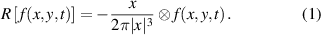
represents the spatial coordinate, and  represents the convolution operator. For the convenience of analysis and solution, the obtained analytical signal is subjected to two-dimensional Fourier transform, which is converted into the wavenumber domain for analysis, and the expression is shown in equation (2),
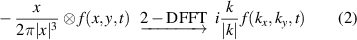
where ![$k = {\left[ {{k_x},{k_y}} \right]^T}$](https://content.cld.iop.org/journals/0964-1726/31/10/105030/revision2/smsac9167ieqn6.gif) represents wavenumber, and
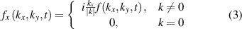
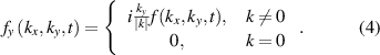
represents wavenumber, and  represents spatial two-dimensional Fourier transform of wavefield signal. After the above Riesz transformation, the imaginary parts
  and
and  in two wavenumber domains corresponding to
  can be obtained, which are defined by equations (3) and (4), respectively,
The first and second transfer functions in the frequency domain are  and
and  , respectively. According to this, the analytical signal in the wavenumber domain can be obtained, which can be represented by equation (5),

where  represents the complex expression of the analytical signal, and
  and
and  represent the orthogonal components of
 ![$R\left[\, {f\left( {x,y,t} \right)} \right]$](https://content.cld.iop.org/journals/0964-1726/31/10/105030/revision2/smsac9167ieqn16.gif) along the x and y directions, respectively.
along the x and y directions, respectively.
Two-dimensional inverse Fourier transform is performed on  , so the signal in wavenumber domain is converted into space-time signal, and the real part
  , imaginary part
  and
and  in space-time domain are restored. After a series of steps, the space-time signal of the original wavefield gets the analytic signal
  of the two-dimensional real signal, which can be expressed by equation (6),

To sum up, the space-time signal of the original wavefield can be transformed by Riesz operator to get the corresponding analytical signal.
2.2. Quality-guided fast phase unwrapping algorithm
The delamination quantification method needs to perform Riesz transform on Lamb wavefield signal to obtain monomorphic analytical signals of wavefield. Then, the spatial distribution of the phase is solved by these analytical signals. Among them, the phase solving process involves the operation of arctangent function, and the phase distribution obtained from the calculation results is truncated to the main value interval of the tangent function, that is, the spatial phase obtained from the solution has a sudden change between −π and π, which can result in phase wrapping. However, the actual phase change should be usually continuous, and the phase distribution should be smooth. To calculate the wavenumber based on the phase, the phase wrapping phenomenon must first be eliminated.
Herráez et al [17] proposed a quality-guided fast phase unwrapping algorithm, which is used to extract the edge contour of the image. The quality-guided phase unwrapping algorithm sets the reliability function for each pixel. To prevent error propagation, the highest quality pixel with the highest reliability value is unwrapped at first, and the lowest quality pixel with the lowest reliability value is unwrapped at last. Therefore, the unwrapping path is determined by using the reliability of pixels.
There are two key problems in the quality-guided phase unwrapping algorithm: the selection of reliability function and the design of unwrapping path. Firstly, for the original phase matrix, the reliability function is transformed into the reliability phase matrix. Then, the quality-guided path is used to unwrap the phases in different positions in turn.
2.2.1. Reliability function.
Quality-guided phase unwrapping algorithm usually defines the reliability based on the gradient or difference between a pixel and its neighbors. If the absolute value of the phase gradient of a pixel relative to its neighbors is greater than 2π, it will be determined as the best point and processed first. However, there are many disadvantages in using the absolute value of gradient in reliability function. For example, if there is a high carrier value, the carrier will become the main modulation component. However, the low carrier value will make the gradient value increase or decrease and produce inappropriate reliability measurement. Second-order difference can solve this problem, and it can provide the measurement of concave/convex degree of phase function, and better detect the possible inconsistency in phase diagram.
Figure 1 is a schematic diagram of the calculation of the second-order difference. Firstly, the reliability function is defined as shown in equation (7), and the phase value of each point is converted into the corresponding value of the corresponding reliability matrix:
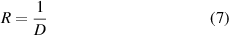
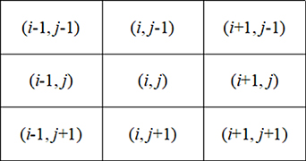
Figure 1. Calculation of second-order difference in matrix.
Download figure:
Standard image High-resolution imagewhere D is defined as,

The parts of the equation are,
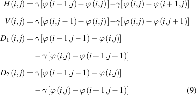
where  represent the phase value, and
  represent adding or subtracting 2π from the phase value.
2.2.2. Unwrapping path.
After solving the reliability matrix, the boundary value between adjacent pixels is constructed, and any pixel with left, right, upper, and lower pixels can construct the boundary. Taking the reliability matrix represented in figure 2(a) as an example, every two orthogonal adjacent pixels have a common boundary. The reliability of this common boundary is defined as the sum of the reliability of two pixels connected by this boundary, as shown in figure 2(b). In the figure, the horizontal boundary is shown in blue, and the vertical boundary is shown in yellow.

Figure 2. Schematic diagram of phase unwrapping path. (a) Reliability matrix, (b) matrix adjacent boundary reliability, (c) adjacent phase unwrapping, (d) regional phase unwrapping, (e) the adjacent phases of the region unwrapping, (f) all phases unwrapping.
Download figure:
Standard image High-resolution imageThe unwrapping path can be defined by observing the reliability value of the boundary. Boundaries are stored in an array and sorted by reliability value. To solve the phase unwrapping problem in the two edges with high reliability, the unwrapping can be carried out in order of reliability. The boundaries with high reliability are unwrapped first, and then the boundaries with low reliability are unwrapped one by one. The reliability matrix shown in figure 2 is taken as an example, the specific unwrapping path can be illustrated by figures 2(c)–(f) until all pixels are unwrapped.
2.3. General flow of delamination imaging
Lamb waves with different excitation frequencies display different wavenumber information when propagating in structures made of different materials, especially for regions with different thicknesses. Therefore, there are significant differences between Lamb waves in healthy and delamination regions, especially at the delamination edge of structures.
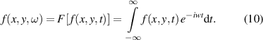
The received space-time wavefield  is usually the result of Lamb waves with a certain frequency bandwidth. To analyze the change of wavenumber of Lamb wave caused by delamination more clearly in the propagation process, this paper uses Fourier transform to extract the single frequency component at a certain characteristic frequency. Firstly,
  is transformed into the frequency domain, and the frequency-space wavefield
  is obtained as shown in equation (10). Then the single frequency spatial wavefield
  at the characteristic frequency
  is extracted.
The Riesz transform is performed on the single frequency spatial wavefield  . The local amplitude value
  , local phase
  and local direction
  of the single frequency wavefield can be expressed as,
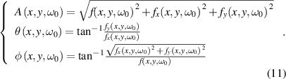
According to the vectorization definition of the monogenic signal, the local amplitude  is the spatial envelope of the original image, and its square is the local energy of the image. The azimuth angle
  represents the local directivity, which describes the local geometric information of the image. The vertex angle
  represents the local phase, which describes the structural information of the image.
From the point of view of phase, wavenumber can be understood as the change rate of phase with distance. Therefore, the wavenumber at any position in space can be obtained from the phase of space-time wavefield,
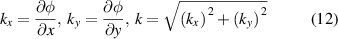
where  represents the wavenumber component in
  direction at spatial position
  ,
,  represents the wavenumber component in y direction at spatial position
  , and
, and  represents the wavenumber value at spatial position
  .
.
Figure 3 is the flow chart of delamination imaging based on Riesz transform, which mainly includes the following main steps,
- (a)Single frequency wavefield signals are extracted from original space-time wavefield signals with a certain frequency band.
- (b)The spatial phase is solved by performing Riesz transform on the single frequency wavefield signal.
- (c)Phase unwrapping is conducted to restore the real space phase.
- (d)The spatial wavenumber distribution is calculated to identify the location, size and shape of delamination.
- (e)The delamination depth distribution is analyzed by the relationship between the wavenumber at the selected frequency and the thickness.
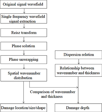
Figure 3. Delamination imaging method based on Riesz transform.
Download figure:
Standard image High-resolution imageComposite laminates are made up of two or more materials with different properties by physical or chemical methods. Because of the difference of material parameters and fiber directions of each ply, the mechanical property and physical parameters of Lamb wave is anisotropic in composite laminates. In order to quantitatively identify the depth information of delamination in composite laminates, it is necessary to calculate the dispersion relation in composite laminates.
Mei et al [18] calculated the dispersion relation of guided waves in composite laminates based on semi-analytical finite element method. According to Lamb wave dispersion relation, the variation of wavenumber with frequency-thickness product of composite laminates can be calculated. When the frequency is constant, the variation relation between wavenumber and effective thickness of composite laminates can be obtained.
According to the calculated wavenumber distribution of composite laminates, the effective thickness of composite laminates can be obtained. The effective plate thickness is equivalent to the depth of delamination, and its calculation method is as follows,
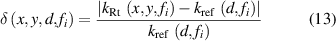

where  represents the calculated spatial wavenumber, and
  represents the wavenumber of a certain thickness
  at a specific frequency
  , which can be found in the thickness-wavenumber curve at the selected mode and frequency.
  represents the error between the spatial wavenumber and the reference wavenumber.
3. Finite element verification
In this section, the finite element simulation method is used to verify the effectiveness of the proposed algorithm for delamination quantification in composite laminates. Firstly, the interaction of Lamb wave and delamination in composite laminates is analyzed and revealed. Secondly, the delamination quantification algorithm based on Riesz transform is studied to identify single and multiple delaminations in composite laminates, and the delamination parameters including location, size, shape, and depth are identified. Finally, the relationship between incident waves along different ply directions and delamination is explored to discuss the effect of delamination imaging, and suggestions on exciting-receiving layout of Lamb wavefield are given for engineering applications.
3.1. Delaminated model of composite laminates
The explicit solution module of ABAQUS is employed to establish the finite element model of Lamb wave propagation. Compared with the implicit dynamic module, the explicit module has a better stability, a faster calculation speed and a lower calculation cost. Delamination is a common damage form in composite laminates and has a great impact on the mechanical properties of the structure. In order to study the interaction between delamination and Lamb wave in the simulation, it is necessary to set a delamination in the model of the composite laminate first. Delamination can be set by node separation at corresponding location. The schematic diagram of the delamination establishment is shown in figure 4. Repeated nodes are set in the upper and lower parts of the delamination area, that is, different nodes are used in the upper and lower elements. This is a common method for modeling delamination in the finite element simulation [19, 20]. In order to analyze the feasibility and accuracy of the delamination quantification algorithm more comprehensively, this paper establishes different delamination cases as shown in table 1. The main purpose of which is to investigate the different performances of the algorithm: (a) identification performance of single and multiple delaminations (case 1 and 2), (b) influence of different incident wave directions on delamination quantification (case 3–6). Figure 5 displays the top view of calculation cases. The delaminations considered here are circular and square.

Figure 4. Schematic diagram of the delamination setup. (a) Without delamination, (b) with delamination.
Download figure:
Standard image High-resolution image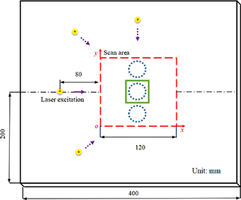
Figure 5. Top view of calculation cases.
Download figure:
Standard image High-resolution imageTable 1. Simulation cases.
| Case number | Incident wave direction | Number of delamination | Delamination size | Delamination depth |
|---|---|---|---|---|
| 1 | 0° | 1 | 30 mm | 0.6 mm |
| 2 | 0° | 3 | 20 mm | 0.6 mm |
| 3 | −90° | 1 | 30 mm | 0.6 mm |
| 4 | −45° | 1 | 30 mm | 0.6 mm |
| 5 | 0° | 1 | 30 mm | 0.6 mm |
| 6 | 45° | 1 | 30 mm | 0.6 mm |
The size of composite laminate is 400 mm × 400 mm × 1.2 mm, and the laminate is made up of six plies with a thickness of 0.2 mm, and the plies are [−45/45/0]s. The material property of each layer is E1= 128 Gpa, E2= 8.2 Gpa, v12= 0.27, v23 = 0.2, G12= 4.7 Gpa, G23= 3.44 Gpa, and ρ= 1560 kg m−3. In different cases, the scanning area is set as a square area with a side length of 120 mm, and the scanning point interval is 1 mm. The boundary condition of the model is fixed around. The element type is C3D8I, and the element size is 0.5 mm, which satisfies the condition that there are more than 10 elements in one wavelength [21].
In general, the total running time of the simulation is determined by the Lamb wave propagation time. The Lamb wave needs to pass through the entire detected area from the beginning to the end, so the total running time of the simulation only needs to be longer than the propagation time of the Lamb wave.
In addition, according to the dynamic theory of the time-domain finite element method, if there are ten elements in one wavelength, the time step Δt needs to satisfy the following condition [22],
where  is the center frequency, and
  kHz in this paper. According to the calculation,
  should be less than or equal to 0.5 μs. In this paper,
  is set as 0.1 μs, which meets the condition.
Therefore, the sampling time interval is set as 0.1 μs, the recording time is 0.5 ms, and there are 5000 steps in total. In the finite element simulation, a node on the upper surface of the model is selected to apply the out-of-plane force signal as excitation, and the out-of-plane displacement of each acquisition point in the sensing area is extracted to simulate the wavefield signal.
In order to avoid the difficulty of delamination quantification caused by high-order modes in Lamb wave propagation, this paper selects five-peak sinusoidal modulation wave with the center frequency of 200 kHz as excitation. At this frequency, only A0 and S0 modes exist in composite laminates. In addition, the out-of-plane displacement mainly includes antisymmetric wave. Therefore, only A0 wave is considered in the model. The expression of the excitation signal is,
where  represents the center frequency of the excitation signal.
3.2. Single delamination quantification
Firstly, the single square delamination model is calculated. Then, the Lamb wavefield in the scanning area is analyzed, and the space-time wavefield snapshots of two selected moments is shown in figure 6. Among them, figure 6(a) shows the wavefield snapshot at 120 μs, when the incident wave encounters the square delamination and has an obvious reflection wave. Figure 6(b) shows the primary wave energy is far away from the delamination at 200 μs.
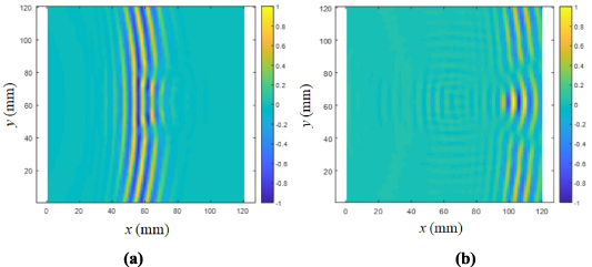
Figure 6. Lamb wavefield in composite laminates with square delamination at (a) 120 μs and (b) 200 μs.
Download figure:
Standard image High-resolution imageThe wavefield with the frequency of 200 kHz is extracted for analysis. From the wavefield shown in figure 7, it can be seen that the Lamb wave with A0 mode at the central frequency changes obviously when it passes through the delaminated area, and there is also obvious trapped wave and scattered wave at the delamination.
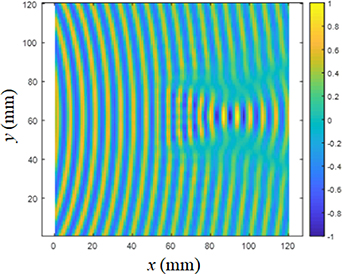
Figure 7. Single frequency wavefield of composite laminates with square delamination at 200 kHz.
Download figure:
Standard image High-resolution imageThe single frequency wavefield is subjected to Riesz transform and monogenic signal processing to obtain the analytical signal, so as to obtain the original spatial phase distribution of the scanned area in the composite laminate. As shown in figure 8(a), the original phase has abrupt changes in many positions, and the phase wrapping is obvious. The quality-guided fast phase unwrapping algorithm is used to obtain the spatial phase distribution as shown in figure 8(b). The phase changes continuously, and the phase corresponding to the delaminated area has an obvious convex shape in the figure. The spatial phase is subjected to partial derivatives in the orthogonal x and y directions, and the wavenumber diagram corresponding to the A0 wave at 200 kHz is further obtained as shown in figure 9. The specific shape of the square delamination and its location in the scanning area can be visually identified from the wavenumber diagram. The wavenumber value of the square delamination area is approximately distributed around 1080 rad m−1, while the non-delamination area is approximately distributed around 900 rad m−1. The black dashed border in the figure represents the theoretical location and shape of the damage. It is observed that the damage identification results are basically consistent with the location and shape of the square damage preset in the model.
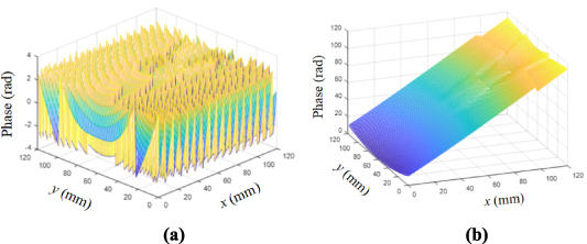
Figure 8. Spatial phase distribution with square delamination. (a) Wrapped, (b) unwrapped.
Download figure:
Standard image High-resolution image
Figure 9. Spatial wavenumber distribution with square delamination.
Download figure:
Standard image High-resolution imageFor a given composite laminate, if the related thickness information is obtained by wavenumber information, the dispersion relation must be calculated and analyzed first. The relationship between thickness and wavenumber at some frequencies can be obtained by using dispersion relation. In the non-delaminated area, the effective thickness is equal to the total thickness of composite laminates. In the delaminated area, the effective thickness corresponds to the depth of delamination, which is less than the total thickness of composite laminates. On account of delamination can only occur between layers, the value of effective thickness is distributed on the thickness values corresponding to different layers, which can also be expressed by the number of layers. The dispersion relation is aimed at the case when Lamb waves propagate at an angle of 0°. Figure 10 shows the schematic diagram of the effective thickness of composite laminates corresponding to the wavenumber of A0 mode at the frequency of 200 kHz, so as to estimate the delamination depth.
According to the figure 10, the delamination depth mapping of the composite laminate with single delamination can be obtained, and the information of the location, size, shape, and depth of the delamination can be intuitively obtained. As shown in figure 11(a), the delamination depth of the square area is around 0.6 mm, which is consistent with the actual delamination location. The depth of the non-delamination area is displayed around 1.2 mm, which is basically consistent with the thickness of the composite laminate. It is worth noting that there is a gradual display at the boundary of the square delamination, and the estimated wavenumber decreases monotonically from the delamination area to the non-delaminated area, thus overestimating the delamination size. This phenomenon is because the propagation process of Lamb wave after delamination is still continuous, and the change of wavenumber is a gradual process. Therefore, it is necessary to select a higher excitation frequency to obtain Lamb wavefield with a smaller wavelength than that of detecting the delamination, to reduce the inaccuracy of the delamination edge as much as possible. According to the estimated depth value in figure 11(a), the depth value at the area y = 60 mm is extracted and compared with the theoretical value. Since the delamination depth should be dispersed at the depths corresponding to different layers, the layers are used for imaging instead of the depth value. As shown in figure 11(b), the red dotted line indicates the theoretical value of layer distribution, the blue solid line indicates the identification result, and the depth value of delamination area is identified at the third layer, which coincides with the theoretical value.
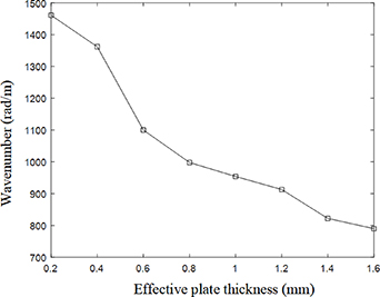
Figure 10. The relation between wavenumber and effective thickness.
Download figure:
Standard image High-resolution image
Figure 11. Imaging results of delamination depth with square delamination. (a) Imaging results, (b) delamination depth curve at y = 60 mm.
Download figure:
Standard image High-resolution imageFurthermore, the differences in calculation time of the three methods are compared. The algorithm of delamination quantification is all completed on the MATLAB platform. The computer is configured with an Intel i5-4590 processor and 16 GB of RAM. For the same original wavefield data containing square delamination, the calculation time of the algorithm proposed in this paper is 1.52 s, while the calculation time of the local frequency-wavenumber domain algorithm and the Hilbert transform algorithm are 65.37 s and 1.44 s, respectively. Compared with the local frequency-wavenumber domain algorithm, the delamination quantification algorithm based on Riesz transform greatly shortens the calculation time. At the same time, under the premise of improving the effect of delamination quantification, the calculation time is almost the same as that of the delamination quantification algorithm using Hilbert transform. In addition, the damage identification method based on the Riesz transform is superior in identifying complex damage shapes [4]. The comparison results of the calculation time of the three methods are shown in table 2.
Table 2. Comparison of calculation time of the three methods.
| Damage identification method | Calculation time |
|---|---|
| Riesz transform | 1.52 s |
| Local frequency-wavenumber domain | 65.37 s |
| Hilbert transform | 1.44 s |
3.3. Multiple delaminations quantification
In practical applications, multiple delaminations may appear in the composite laminates, which are distributed in different locations. In this section, the identification ability of delamination quantification algorithm in multiple delamination scenarios is further studied, mainly focusing on multiple delaminations in composite laminates.
The model simulation results of the composite laminates with multiple delaminations are shown in figure 12. Figure 12(a) shows the Lamb wavefield in the sensing area at 140 μs, and figure 12(b) shows the Lamb wavefield at 160 μs when the Lamb wave passes through the delamination. It can be observed that Lamb wave has obvious trapping and scattering when it encounters delamination at different locations. Figure 13 shows the dominant frequency wavefield extracted by Fourier transform at 200 kHz. In the single frequency Lamb wavefield, Lamb wave interacts with different delaminations, which makes the propagation of Lamb waves more complicated than single delamination.
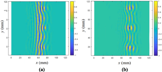
Figure 12. Lamb wavefield of multiple delaminations at (a) 140 μs and (b) 160 μs.
Download figure:
Standard image High-resolution image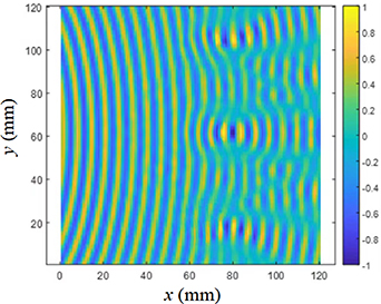
Figure 13. Single frequency wavefield with multiple delaminations at 200 kHz.
Download figure:
Standard image High-resolution imageFigure 14 shows the spatial phase solved by the single frequency wavefield of the dominant frequency. It can be seen from the figure that the spatial phase has a more obvious display in the area of the preset delamination. The spatial wavenumber imaging results obtained by the delamination quantification algorithm are shown in figure 15(a). The black dashed boxes in the figure represent the location and contour of the preset delamination, respectively. The identified delamination location, size and shape basically coincide with the preset delamination. Combined with the dispersion relationship in figure 10, the result of delamination depth quantification is shown in figure 15(b). The delamination depth of the delamination area is about 0.6 mm, which is basically consistent with the preset value, and the preset three delaminations have been well identified.
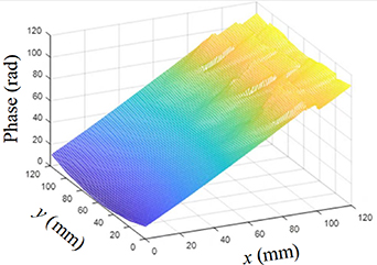
Figure 14. The spatial phase of the wavefield after unwrapping.
Download figure:
Standard image High-resolution image
Figure 15. Multiple-delamination imaging. (a) Spatial wavenumber, (b) delamination depth.
Download figure:
Standard image High-resolution image3.4. Influence of incident wave direction
The anisotropy of the composite materials affects the propagation and scattering of Lamb waves in the structure. Therefore, Lamb waves in different incident directions can be used to scan the structure, which may affect the identification effect of the delamination quantification algorithm in the composite laminate. Therefore, this section studies the interaction between Lamb wave and delamination when it is incident from different directions and explores the identification effect of delamination quantification algorithm in different incident wave directions. As shown in case 3–6 in table 1 and figure 5, four excitation points representing different incident directions of Lamb waves are respectively set on the composite laminate with a circular delamination. The directions of the incident waves are −90°, −45°, 0° and 45° respectively relative to the scanning area.
The spatial wavefield signals of Lamb waves with different incident directions are acquired and analyzed. Figure 16(a) shows the spatial wavefield snapshot when the Lamb wave propagates to the circular delamination in the incident direction of 45°. It can be seen that the delamination at this moment introduces a strong forward scattering wave, which even submerges the normal scattering phenomenon of delamination. Figure 16(b) shows the spatial wavefield snapshot when the Lamb wave incites from the direction of −45°. An obvious forward scattering wave at the delamination can be also observed. Figures 16(c) and (d) respectively show the spatial wavefield snapshot when the Lamb wave incites from the direction of 0° and 90°. The trapping and scattering of the Lamb wave can be clearly seen from the figures, and there is no forward scattering wave different from that in figures 16(a) and (b).
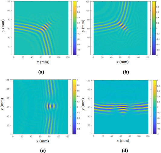
Figure 16. Spatial wavefield under different incident wave directions. (a) 45°, (b) −45°, (c) 0°, (d) −90°.
Download figure:
Standard image High-resolution imageSingle frequency wavefield signals with different incident directions at 200 kHz are extracted and analyzed. As shown in figures 17(a)–(d), it can be observed from the single frequency wavefield that Lamb wave has an obvious energy focusing in the incident directions −45° and 45°, which even leads to almost invisible trapping and scattering at the delamination. The forward scattering wave in figures 16(a) and (b) is also caused by the energy focusing along −45° and 45°, which are the orientations of outermost and sub-outer fibers, respectively. Conversely, in the single frequency wavefield in the incident direction of 0° and 90°, the Lamb wave scattering and trapping in the delaminated area of the wavefield are normal and obvious.

Figure 17. Single frequency wavefield under different incident directions. (a) 45°, (b) −45°, (c) 0°, (d) −90°.
Download figure:
Standard image High-resolution imageThe central frequency wavefields in different incident directions are analyzed and the spatial phase is solved in figure 18. The spatial phase diagrams under incident directions −45° and 45° are not prominent in the delaminated area, and the delamination cannot be observed intuitively. By contrast, the spatial phase diagrams under incident directions −90° and 0° show that the phase amplitude of the delaminated area is quite different from that of the non-delaminated area.
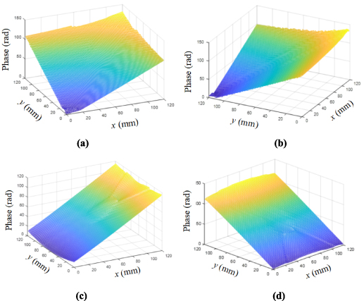
Figure 18. Spatial phase of composite laminates under different incident directions. (a) 45°, (b) −45°, (c) 0°, (d) −90°.
Download figure:
Standard image High-resolution imageThe wavenumber distribution can be solved and shown in figure 18. It can be seen from figures 19(a) and (b) that the wavenumber distribution is very disordered and it is difficult to distinguish the position, shape and size of the delamination, which is caused by the energy focusing phenomenon along the directions −45° and 45°. Conversely, figures 19(c) and (d) give good identification results of the delamination parameters, including location, size, and shape.
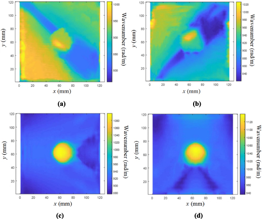
Figure 19. Spatial wavenumber distribution under different incident directions. (a) 45°, (b) −45°, (c) 0°, (d) −90°.
Download figure:
Standard image High-resolution imageIt can be seen from the above analysis that when the angle between the excitation points and the signal acquisition area (incident wave angle) is 45° or −45°, that is the directions of outermost and sub-outer fibers, the delamination imaging quality is poor. On the contrary, when the angle between the excitation point and the signal acquisition area (incident wave angle) is 0° and −90°, the delamination quantification algorithm gives a good identification result.
It can be seen that the delamination quantification is adversely affected when the incident wave direction is along the outer fiber direction. The main reason is that the layup of the composite laminate is [−45/45/0]s, and the energy accumulation of Lamb waves occurs at the outermost surface 45° and the sub-outer surface −45°, which drowns out the original scattering phenomenon. Therefore, strong forward scattered waves appear at the location of delamination, resulting in inaccurate identification results.
In summary, it can be concluded that when setting the scanning path and the excitation point, it is essential to avoid the situation that the incident wave direction completely coincides with the direction of the outermost and sub-outer fibers, which can be realized by setting the relative position between the scanning area and the excitation point.
4. Experimental verification
A non-contact laser ultrasonic detection system has been set up to obtain Lamb wavefield signals of composite laminates and further verify the accuracy and effectiveness of the proposed delamination quantification algorithm.
4.1. Experimental setup
The experiment systems consist of pulse laser, laser interferometer, data acquisition card, two-axis linear scanning device, controller, and other equipment, which are shown in figure 20(a). In the aspect of signal excitation, Nd:YAG pulse laser is used for excitation. The laser wavelength is 1064 nm, the pulse width is 10 ns, and the maximum energy of a single excitation pulse can reach 55 mJ. In the aspect of signal acquisition, double-wave mixing interferometer AIR-1550-TWM is used for signal acquisition. The wavelength of continuous laser is 1550 nm, and the minimum spot radius can reach 200 μm. The principle of signal acquisition of laser interferometer is the interference of original light and reflected light from the sample surface. In addition, the laser receiving probe is installed on the two-axis linear scanning rack, and the precise movement and positioning of the probe position are controlled by the computer cooperatively, so as to complete the data acquisition of the scanning area by the probe according to the preset path. The schematic diagram of the laser ultrasonic detection system is shown in figure 20(b).
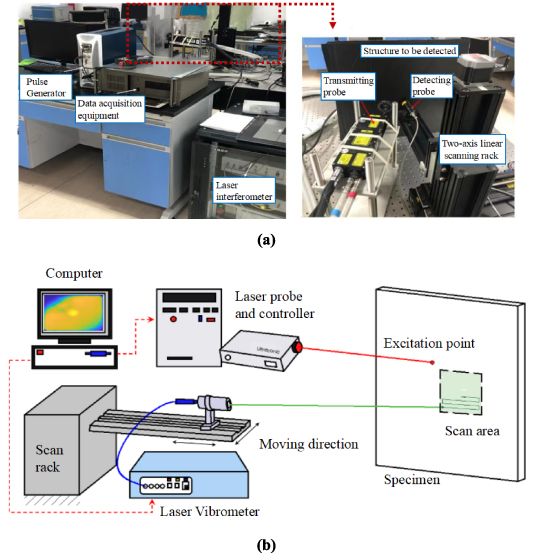
Figure 20. Experimental platform and schematic diagram of laser ultrasonic testing system. (a) Experimental platform, (b) schematic diagram.
Download figure:
Standard image High-resolution image4.2. Specimen and scanning scheme
The dimensions of the composite laminate are 400 mm × 400 mm × 1.2 mm. It is made of the T300 prepreg, which as shown in figure 21(a). The material property of each layer is E1= 139.9 Gpa, E2 = 10 Gpa, v12= 0.3, v23 = 0.47, G12= 5.7 Gpa, G23 = 3.41 Gpa, ρ = 1560 kg m−3. The ply direction is [−45/45/0]s. A circular polyimide film with a diameter of 20 mm is placed at a preset position between the layers to model the circular delamination in the experimental specimen. The composite laminate consists of six plies, and the delamination is placed between the third ply and the fourth ply, which indicates that the delamination depth is 0.6 mm.
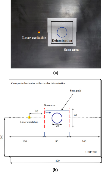
Figure 21. Specimen diagram and scanning scheme for the delamination quantification in composite laminates. (a) Specimen diagram, (b) scanning scheme.
Download figure:
Standard image High-resolution imageThe horizontal and vertical space intervals of each scanning point in the scanning area are both set as 1 mm. In the experiment, the single pulse energy of laser is set as 16 mJ, and the laser excitation and receiving beams are perpendicular to the composite laminate. The measuring head of the interferometer moves and covers the detection area according to the set bow-shaped scanning track, as shown in figure 21(b).
4.3. Experimental result analysis
By combining the Lamb wave signal acquired by the interferometer with the location information provided by scanning frame, a time-space-amplitude matrix representing Lamb wavefield can be obtained. As can be seen from figure 22, Lamb wave gradually propagates from the excitation point to the delamination. Figures 22(a) and (b) show the Lamb wavefield snapshots at 100 μs and 200 μs, respectively. The wavefield clearly shows trapped wave and scattered wave in the delaminated area.

Figure 22. Lamb wavefield at (a) 100 μs and (b) 200 μs.
Download figure:
Standard image High-resolution imageAs shown in figure 23, the single frequency wavefield at 120 kHz is extracted from the original wavefield data. The signal is acquired by the out-of-plane displacement of the composite laminate. Therefore, the wave mode is A0 mode.
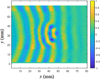
Figure 23. Single frequency wavefield of composite laminates at 120 kHz.
Download figure:
Standard image High-resolution imageThe spatial phase of the single frequency spatial wavefield signal is solved by Riesz transform, and the unwrapped spatial phase is shown in figure 24(a). Similar as in the simulation, the phase distribution in the delaminated area has an obvious convex trend compared with the non-delaminated area. The spatial wavenumber distribution obtained from the spatial phase is shown in figure 24(b), in which the black dotted line indicates the preset location and shape of the delamination. In the preset delaminated area, that is, the wavenumber value is obviously higher than that in the non-delaminated area. Delamination parameters such as location, size and shape in the specimen can be obtained by observing the wavenumber diagram.
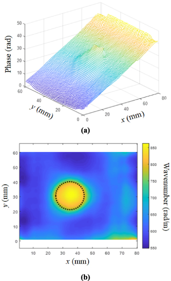
Figure 24. Spatial phase and wavenumber distribution in the composite laminate. (a) Spatial phase, (b) spatial wavenumber.
Download figure:
Standard image High-resolution imageCombining the material properties, the dispersion relation between effective plate thickness and wavenumber is obtained as shown in figure 25. Comparing the spatial wave value with the thickness-wavenumber curve obtained by dispersion curve, the spatial effective thickness in the scanning area is obtained. Figure 26 shows the outline and depth information of the delamination. The delamination depth is around 0.7 mm, and the thickness of the non-delaminated area is around 1.4 mm. The experimental results show that the proposed delamination quantification algorithm can accurately identify the delamination location, size, shape and depth.
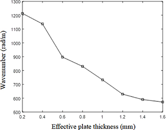
Figure 25. Relationship between wavenumber and effective thickness of composite laminates.
Download figure:
Standard image High-resolution image
Figure 26. Effective depth distribution of composite laminate.
Download figure:
Standard image High-resolution image
5. Conclusions
In this paper, the feasibility and effectiveness of monogenic signal-based delamination quantification algorithm in the composite laminates are studied and verified by finite element simulation and experiment.
- (a)The delamination quantification algorithm proposed in this paper can effectively detect the location, size, shape and depth of delamination in composite laminates. This method has the advantages of high recognition accuracy and short calculation time.
- (b)There may be more than one delamination in the composite material. In response to this situation, the algorithm proposed in this paper can not only identify single delamination in composite laminates, but also identify multiple delaminations at the same time.
- (c)This paper also discusses the interaction between Lamb waves and delamination in different incident wave directions, and studies the influence of delamination quantification from the incident wave directions. The results show that it is necessary to avoid the same direction with outermost and sub-outer fibers when setting the excitation point and scanning area. Its reason and solution deserve a special and further study.
In future, some important and further works may be considered as follows:
- (a)In practical engineering, due to the large process discreteness of composite materials, the uncertainty of material parameters and thickness will affect the quantification of damage. How to eliminate this effect is indeed a very interesting and useful topic. Future research in this area can be carried out to solve this problem.
- (b)The application of impact damage quantification algorithm based on monogenic signal can be further studied. Moreover, the detection capabilities of the algorithm in more complex structures, such as composite stiffened panels, can be further explored.
Acknowledgments
This research was supported by the projects from the Natural Science Foundation of China (Grant Nos. 11902280 and 12272331), China Prostdoctoral Science Foundation (Grant No. 2021M700872), Aeronautical Science Fund (Grant No. 20200033068001), the Natural Science Foundation of Fujian Province (Grant No. 2022J01059), Innovation Foundation for Young Scholar of Xiamen (Grant No. 3502Z20206042) and the Fundamental Research Funds for the Central Universities (Grant No. 20720210049).
Data availability statement
The data generated and/or analysed during the current study are not publicly available for legal/ethical reasons but are available from the corresponding author on reasonable request.