
Abstract
Vibration energy harvesting has been a popular topic in recent years. This technology is promising in developing self-powered sensor nodes for health condition monitoring of machines or structures, especially in remote areas. This study proposes a pendulum-flywheel vibration energy harvester based on the electromagnetic energy conversion mechanism. The harvester has two motion modes, namely the pendulum mode and eccentric flywheel mode, and can switch between the two modes automatically in response to external excitations.
We first establish a theoretical model and fabricate a prototype of the harvester for evaluating its performance. Then, experimental and theoretical methods are employed to estimate the parameters of the model, such as the dipole moment of magnets, the mechanical damping coefficients, and the optimal resistance of the external electrical load. The typical trajectories of different motion modes, the frequency response characteristics, and the influence factors on the basins of attraction of the harvester are studied with the theoretical model. It is found that the small magnet distance can broaden the frequency band and enlarge the amplitude of the dynamic responses of the system. This finding provides us with an approach to control the performance of harvester and enables it to have stronger adaptability to variant ambient vibration in nature. Finally, laboratory tests are performed to validate the theoretical model. The experimental data verified the assumption that the rotation speed of the pendulum and the induced electromotive voltage have a linear relationship. Experimental and numerical simulation results show that the errors between them in most cases are less than 10% when the excitation displacement is small and have a slight increase with the excitation displacement. In the experiments, this harvester achieves a maximum power of 16.3 mW, exhibiting good performance in comparison with the-state-of-the-art pendulum-based harvesters.
Export citation and abstract BibTeX RIS
1. Introduction
The rapid development of communication and sensing technologies make low-power sensors and communication equipment possible [1]. These low-power and high-efficiency devices enable us to set up self-powered autonomous systems, such as wireless sensor networks, using energy harvested from the ambient environment. Self-powered solutions are capable of overcoming the issues brought about by the limited service life of batteries and the vulnerability of electric cable networks, especially in remote areas [2]. Thus, energy harvesting technologies used for self-powered systems have been a popular topic recently.
Energy harvesting is a process of converting the local naturally available energies to electricity for local use [3]. Mechanical energy, thermal energy, light energy, and chemical energy can all be employed as sources for energy harvesting [2]. Mechanical vibration has gained more attention due to its abundance in nature [4]. Various transduction mechanisms for vibration-based energy harvester, such as piezoelectric [5–9], electromagnetic [10–14], electrostatic [15], and magnetostrictive [16], triboelectric [17] have been reported. Piezoelectric [18–20] and electromagnetic [21–24] mechanisms or the hybrid of both mechanisms [25–27] are the most commonly exploited in macro vibrational energy harvesters (VEHs). Electromagnetic VEHs scavenge vibrational energy via Faraday's law of induction, whereas energy generation by piezoelectric harvesters is proportional to the strain in piezoelectric materials. Piezoelectric harvesters are sensitive even at small vibrational amplitudes and tend to work well in the high-frequency range [28]. However, the internal resistance of piezoelectric materials limits the energy conversion efficiency of piezoelectric harvesters. Compared with piezoelectric harvesters, electromagnetic ones are mainly employed in larger-scale applications and can output considerable energy in the low-frequency range [11].
According to the frequency-response characteristics, known energy harvesters can be categorised into three groups: single frequency-based systems, multiple frequencies-based linear systems, and broadband-based nonlinear systems [29]. For linear systems, the output power reaches the maximum at resonance and reduces dramatically at other non-resonating frequencies [12]. This limitation has led to the work of developing multiple frequencies-based and broadband-based energy harvesters. Multiple frequencies-based harvesters generally use a generator array, each of which has a different resonant frequency, to achieve widening bandwidth [30]. Such a design enables the harvesters to extract energy efficiently at multiple frequencies.
Besides, introducing nonlinearity to harvester systems is a more efficient but sophisticated solution to harvest energy from a continuous frequency band [31]. The energy potentials of nonlinear energy harvesters typically have multiple wells. When moving from one potential well to another, the system has large deformations or displacements and consequently harvesting more energy [32]. In practice, the nonlinear magnetic force or large deformation of structures is often used for providing nonlinearity to energy harvesting systems [33, 34]. This principle has been widely utilised in both electromagnetic and piezoelectric energy harvesters. For example, the authors have developed a multi-stable electromagnetic harvester using the nonlinear magnetic force for broadening the response-frequency band and increasing the output energy [11].
Different harvesters have different structures, and each configuration has its advantages and suits specific conditions. Among all the structures exploited in designing VEHs, spring-mass like structure [35], cantilever beam [10], and pendulum [32] are very popular. For spring-mass systems, energy can be scavenged from the reciprocating motion of the mass under operational conditions. Such systems usually work well at resonance, but the introduction of nonlinear restoring force can broaden the bandwidth of resonant frequency. Spring-mass like structures are common in electromagnetic harvesters.
Compared with a spring-mass structure, a cantilever beam is more common in both electromagnetic [36] and piezoelectric [18] VEHs because of its more straightforward structure. A cantilever-beam structure having no movable components makes it easier to fabricate. Under the action of external excitation, stress and strain are generated inside the beam. Electricity is generated via the strain of a cantilever beam in piezoelectric VEHs, and via the displacement at the free end of a beam in electromagnetic VEHs.
Although the advantages of a cantilever-beam structure are outstanding, some of its limitations must not be overlooked. Cantilever structures are prone to damage due to stress concentration at the fixed end of the beam. Besides, tip mass or other accessories are needed to enrich the dynamic behaviours of the system. A pendulum, having a simple design principle, can exhibit complex dynamic behaviours. Pendulum-based VEHs can change from a linear to a nonlinear system automatically with the increase of excitation levels. This feature allows a pendulum-based VEH to adapt to more complex excitation conditions. Consequently, a pendulum-based structure is also common in the design of VEHs [1, 12, 37, 38]. Sometimes, a combination of different structures performs better by taking advantages of each structure [39].
Recently, some studies on bi-stable rotational energy harvesters have been reported. For instance, Han et al [40] proposed a bi-stable structure which comprised a simple pendulum linked with a linear spring. The nonlinearity of this system mainly came from the large angular displacement of the pendulum. Some other studies made use of a magnetic force to provide nonlinearity to bi-stable energy harvesting systems [41–43]. Kim et al [43] put forward a bi-stable harvester composed of two magnetic-coupled piezoelectric cantilever beams for facilitating the energetic inter-well response for relatively low excitation amplitudes and frequencies in multiple directions. Fu et al's rotational harvester [41] consisted of a piezoelectric cantilever beam with a tip magnet interacting with another magnet attached on the rotating host. This harvester had a bi-stability and frequency up-conversion characteristic for harnessing low-frequency kinetic energy with a wide bandwidth. Compared with other reported VEHs, the nonlinearity of the pendulum-flywheel VEH in this work originates from both magnetic repulsion and large angular displacements. These complex nonlinearities enable this harvester to have time-variant dynamic behaviours. Besides, the proposed VEH can shift between the pendulum and flywheel modes automatically in response to excitation, which presents a passive mechanism. Such a passive mechanism endows the pendulum-flywheel harvester stronger adaptability to various excitations and enhances its energy harvesting performance in a broader frequency range. Although the dynamics of bi-stable harvesters have been studied widely, the proposed pendulum-flywheel structure has distinct dynamical behaviours.
The contributions of this work are summarised as follows:
(1) To our best knowledge, a pendulum-flywheel VEH based on the electromagnetic mechanism is first proposed in this paper. Although a small number of papers also reported VEHs with both a pendulum and a flywheel, e.g. in [4], and [38], these VEHs swing in a small angular range and operate on only a pendulum mode. Our proposed pendulum-flywheel structure can not only oscillate around its stable equilibrium point, but also rotate to harvest more energy, that is, it has both pendulum and flywheel modes, and can automatically switch between them in response to the intensity of excitations. This feature endows this device strong adaptability to various ambient vibrations.
(2) A theoretical model of this pendulum-flywheel VEH is established based on the D'Alembert's principle and Kirchhoff's Voltage Law.
(3) An approach to controlling the nonlinearity of the harvester by adjusting magnet distance is suggested. This approach makes the pendulum-flywheel more adaptive to various application scenarios.
This study carries out a series of investigations on the harvester's structural dynamics behaviours and efficiency for harvesting more energy. The remainder of this paper is organised as follows: section 2 introduces the concept of the pendulum-flywheel energy harvester. Subsequently, section 3 presents the establishment process of the theoretical model of the proposed VEH. Section 4 describes the fabricated prototype of the harvester. Estimation and verification of model parameters are conducted in section 5. In section 6, a numerical analysis of the VEH's dynamical behaviours is made. Section 7 provides the experimental verification of the proposed theoretical model. Finally, conclusions are drawn according to the relevant analysis.
2. Concept of the pendulum-flywheel VEH
Figure 1 shows the schematic diagram of the proposed pendulum-flywheel VEH, composed of a frame, two magnets, a fan-shaped pendulum, an annular gear, a pinion gear, and a DC generator. The frame of this harvester is fixed on a base plate that receives excitations. The fan-shaped pendulum is connected to the frame through a rotating shaft. The annular gear and fan-shaped pendulum are bolted together and share the same centre of rotation. The pinion gear meshes with the internal teeth of the annular gear and is connected to the rotating shaft of the DC generator by an interference fit. The DC generator is fixed to the frame of the VEH. Driven by the swinging fan-shaped pendulum, the annular gear rotates around its centre of rotation to turn the pinion gear which in turn drives the DC generator to convert mechanical energy to electricity.
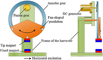
Figure 1. Schematic of the pendulum-flywheel energy harvester.
Download figure:
Standard image High-resolution imageThe DC generator produces electrical power based on Faraday's law of electromagnetic induction. The essential parts of a DC generator include a stator, a rotor, armature windings, a yoke, poles, pole shoes, a commutator, and brushes. The rotor includes a cylindrical armature core stacked with slotted iron laminations. Armature windings (coils) are in a closed circuit form and connected in series for enhancing the voltage outputs. The stator is utilised for providing a magnetic field in which the coil spins. The poles are used to hold the field windings and the pole shoes to spread the magnet flux for avoiding the field coil from falling. A commutator can work as a rectifier to change the voltage within the armature windings from AC to DC. The brushes are employed to realising the electrical connection between the commutator and exterior load circuit. Driven by the pinion gear being turned by the pendulum-flywheel mechanism, the rotor and armature windings rotate in the magnetic field, generating an alternating voltage. However, a unidirectional voltage can be obtained with the commutator and brushes.
The fixed magnet is attached to the base of the harvester frame and moves with it. The tip magnet is stuck on the bottom rim of the fan-shaped pendulum. The repulsion between magnets acts on the fan-shaped pendulum through the tip magnet. The nonlinear magnetic force induces a bi-stable potential function, being helpful to broaden the frequency band of the system. This VEH has two motion modes, namely the pendulum and flywheel modes, to adapt to different magnitudes of horizontal base excitations. The fan-shaped structure swings as a pendulum when subjected to weak excitations. On the other hand, the fan-annular gear-tip magnet assembly rotates around the centre of rotation continuously, becoming an eccentric flywheel, when subjected to intense base excitations. This harvester switches from one mode to another automatically according to the magnitude of base excitations, enabling this VEH to have stronger adaptability to variant excitations in nature.
3. The theoretical model of the proposed VEH
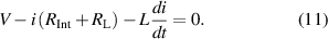
Based on the proposed concept, a theoretical model of the VEH is established in this section. Calculating the recovery torque of the system is one of the most critical steps while building the dynamical model of the VEH. The magnetic repulsion and gravity work together to generate the recovery torque of this harvesting system. The gravity is a volume force which does not change with the position of objects. The recovery torque by gravity can be calculated as follows:

where  is the mass of the pendulum system, including the fan-shaped structure, the bolts, the tip magnet, and other accessories;
  is the local gravity of the Earth;
  stands for the distance between the centre of gravity and the centre of rotation;
  is the angular displacement of the fan-shaped structure. The recovery torque by gravity
  only depends on the force arm
  . However, calculating the torque by magnetic repulsion is more complex, as the magnetic force has strong nonlinearity.
Usually, the magnetic repulse between two magnets can be obtained through an analytical method [44], a numerical method [45], or an experimental method [46]. An analytical method is used to express the repulsion between fixed and movable magnets, which leads to the recovery torque  due to magnetic force below:

where  denotes the component of magnetic force in the moving direction of tip magnet;
  is the radius of the fan-shaped pendulum. By simplifying these permanent magnets as two dipoles,
  can be expressed as follows [44, 47]:
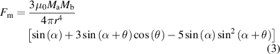
where  is the permeability of free space, which has an exact value of 4
 E-7
E-7  ;
;  and
and  are the magnetic dipole moments of the two magnets;
  is the distance between the centres of the two magnets.
 is a function of
  ,
,  , and
, and  , which can be written as:
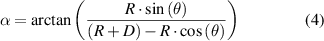
where  is the distance between the tip and fixed magnets when the angular displacement
  equals 0. The definition of some critical variables is presented in figure 2. By substituting equation (3) into equation (2), the recovery torque by magnetic force can be derived.
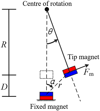
Figure 2. Definition of some critical variables.
Download figure:
Standard image High-resolution imageFigure 3(a) describes the force diagram of the pendulum-flywheel VEH. For simplifying analysis, this harvester is divided into two subsystems, namely, the inertial-motion subsystem and the energy-conversion subsystem. The inertial-motion subsystem includes the fan-shaped pendulum, the annular gear, and the tip magnet. The energy-conversion subsystem is composed of the pinion gear and the DC generator. According to D'Alembert's principle, the dynamic equation of the inertial-motion subsystem can be written as follows:


Figure 3. Physical model of the harvester: (a) the force diagram; (b) the equivalent circuit.
Download figure:
Standard image High-resolution imagewhere  stands for the equivalent polar moment of inertia of the inertial-motion subsystem;
  is the mechanical damping coefficient of this system;
 is the angular position of the fan-shaped structure;
  and
and  are the recovery torques by magnetic force and gravity;
  denotes the acceleration of the horizontal base excitation, which is a function of time
  ; the term
  stands for the torque caused by base excitation and is the function of
  and
and  . The two variables,
  and
and  , make the VEH's dynamical characteristics more complex;
  represents the tangential component of the interaction force between the annular gear and the pinion gear, and
  the radius of the pitch circle of the annular gear. The equation of motion of the energy-conversion subsystem is:

where  is the equivalent polar moment of inertia of the energy-conversion subsystem;
  stands for the angular displacement of the pinion gear, equal to the angle of rotation of the DC generator;
  is the mechanical damping coefficient of the energy conversion subsystem,
  the radius of the pitch circle of the pinion gear;
  stands for the torque by the generator, which is proportional to the electrical current
  with a torque constant
  [48, 49],

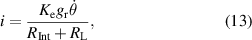
As the pinion and the annular gears engage with each other, there is a constant gear ratio  between them,
According to the relationship between the tooth number and the radius of the gear  , equation (8) can also be written as follows:
The back electromotive voltage  of the generator is proportional to the rotational speed
  of the rotor of the generator [4], which can be written as:

where  is the back electromotive force constant.
For converting the electromotive voltage into electricity, the generator needs to be connected to a closed circuit, which has an external electrical load. The equivalent circuit of the harvester is shown in figure 3(b), where  is the internal resistance of the generator, and
  the inductance of this closed circuit;
  is the current generated in this circuit due to the electromotive voltage of the generator, and
  represents the resistance of the external electrical load. Applying Kirchhoff voltage law for the circuit, one obtains:
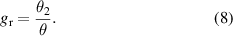
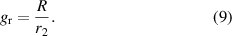
Since the pendulum-flywheel VEH is expected to usually operate at low frequencies, neglecting the inductance  has little impact on the performance of the electric circuit [49]. Thus, equation (11) can be rewritten as follows:

The inductance  of the DC generator is estimated to be below and near 3.2
  . Numerical simulation results of several examples with L = 3.2 mH and L = 0 indicate that
  can be neglected in equation (11), that is, equation (12) can be used, without any noticeable loss of accuracy. Based on equations (7), (8), (10), and (12), the current
  and torque of the generator
  are obtained:
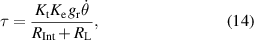
Substituting equations (6), (9), and (14) into equation (5), the dynamical model of the inertial-motion subsystem can be derived as:
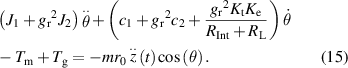
Both  and
and  are functions of angular position
  and have a nonlinear characteristic. However, the pendulum oscillates with a small amplitude of angular displacement when subjected to a weak excitation, which can be approximately regarded as a linear system. Therefore, the natural frequency of the corresponding linear system can be estimated as:
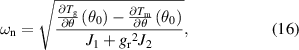
where  and
and  are the partial derivative of
  and
and  with respect to variable
  , corresponding to the stiffness of the system caused by magnetic force and gravity when
  ;
;  denotes the stable equilibrium point of the pendulum structure. The value of
  varies with numerous factors, such as the mass of the pendulum and the position of the fixed magnet. Estimating the natural frequency of the system provides an insight into the dynamic characteristics of the harvester. Besides, the instantaneous power generated by
  is
is
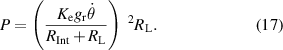
With equations (15)–(17), we are able to investigate the dynamic behaviours of the pendulum-flywheel VEH and estimate its energy performance.
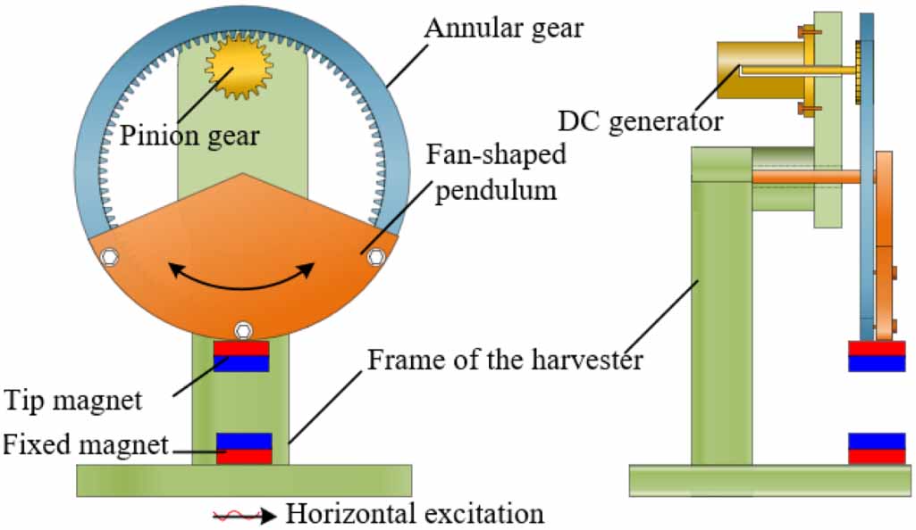
4. The prototype of the VEH
According to the concept of the proposed pendulum-flywheel VEH, a prototype is designed and fabricated, as shown in figure 4. Both the frame and the annular gear are built through a 3D-printing process with nylon. The fan-shaped structure, the pinion gear, and the washer are made of aluminium. The fan-shaped structure has a central angle of 130° and a thickness of 2 mm. Two identical cylindrical neodymium magnets (grade number: N52; size: mm) are employed in the prototype. Different from the schematic diagram in figure 1, we also attach a nylon fixture on the fan-shaped structure to provide the block of mass with space for installing additional masses (if needed). The block of mass (material: copper, size:
  mm) is used for obtaining a larger inertial force. Considering the block of mass and nylon fixture as parts of the inertial-motion subsystem, the proposed theoretical model still works. The DC generator is installed on the Nylon frame through a 3D-printed fixture and connected to a close circuit via the wire connector. Since the fixed magnet is mounted on the frame foot, the distance between the tip and fixed magnets can be adjusted by moving the vertical position of the rotating shaft of the pendulum to a different position on the frame. Some detailed parameters about the prototype, including the magnets and DC generator, are presented in table 1. However, the magnetic dipole moment of magnets and the mechanical damping coefficient of the VEH cannot be obtained directly. They are determined from experimental data.
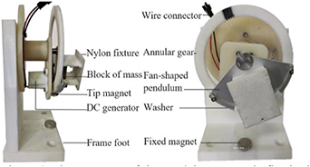
Figure 4. The prototype of the pendulum-eccentric flywheel VEH (left: side view; right: front view).
Download figure:
Standard image High-resolution imageTable 1. Parameters of the designed prototype.
| Parameter | Value | Unit | Parameter | Value | Unit | ||||
|---|---|---|---|---|---|---|---|---|---|
| VEH |

| 2.48E-4 |

| Permanent magnet | Diameter | 20 |

| ||

| 9.88E-8 |

| Height | 8.7 |

| ||||

| 1.96E-2 |

| Magnet Grade | N52 | |||||

| 5.72E-2 |

| Magnetisation Direction | Axial | |||||

| 110.02E-2 |

| Weight | 11.90 |

| ||||

| 3.32E-2 |

| Surface field | 2999 |

| ||||

| 6.00E-2 |

| Maximum operating temperature | 80 | °C | ||||

| 5.20E-3 |

| Remanence | 14 700 | Gauss | ||||

| 9.23 | Maximum energy product | 52 | MGOe | |||||
| Teeth number-annular gear | 120 | DC generator | Induced voltage | 1–5 |

| ||||
| Teeth number-pinion gear | 13 | Internal resistance ( ) ) | 94 |

| |||||
| Standard pressure angle | 20 |

| Rated speed | 500 |

| ||||
| Addendum | 8.00E-4 |

| Rated torque | 10 |

| ||||
| Tooth length | 1.80E-3 |

| Rated current | 50 |

| ||||
| The radius of the fan-shaped structure | 3.85E-2 |

| Rated power | 150 |

| ||||
| The central angle of the fan-shaped pendulum | 130 |

| Rotation direction | CW/CCW | |||||
5. Estimation and verification of model parameters
In this study, we use a series of experiments to estimate magnetic dipole moments  and
and  , and damping coefficients
  and
and  . Comparisons between the calculated and experimental recovery torques of the system are conducted to verify the effectiveness of the analytical model. Besides, we discuss the optimal resistance of the electrical load through numerical simulations.
5.1. Estimation of the magnetic dipole moments
As two identical permanent magnets are used in the prototype, magnetic dipole moments  and
and  share the same value. According to equation (3), we know
  is a function of magnetic dipole moments
  and
and  , allowing us to estimate the dipole moments with different magnetic forces. To achieve such a goal, magnetic forces in the vertical direction are measured with the experimental setup shown in figure 5(a), where the angular position
  is fixed to 0 for simplifying experiments. Then, the least-squares fitting method is used to determine the optimal
  and
and  . When
  , the magnetic force calculated by equation (3) fits best to experimental data, as shown in figure 5(b).
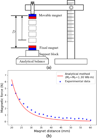
Figure 5. Estimation of the magnetic dipole moments: (a) experimental setup; (b) curve fitting results.
Download figure:
Standard image High-resolution image5.2. Estimation of the mechanical damping coefficients
An experimental approach is adopted in this study to estimate the damping coefficients  and
and  , the setup of which is shown in figure 6(a). A Bluetooth-version gyroscope module (WT901B, by WitMotion Shenzhen Co., Ltd) is fixed on the centre of rotation of the pendulum-flywheel structure to record its dynamic behaviours. This sensor module, integrating the high-precision gyroscopes, accelerometers, and geomagnetic sensors, has a maximum sampling frequency of 200 Hz. By fusing the multiple attitude data through a dynamic Kalman algorithm, the precision of gesture resolution is up to 0.01 degrees. These gesture data can be transmitted to the computer in real-time via the USB Bluetooth adapter. We design two cases to estimate damping coefficients
  and
and  , respectively. In case 1, the energy-conversion subsystem, including the pinion gear and the DC generator, is removed from the VEH. Then, the inertial-motion structure is released from the angular position of 0.5
 and swings freely under the influence of gravity and the mechanical resistance related to
  . The simulated curve fits well to experimental data when
  =2.5 × 10⁻⁴
 . In case 2, the energy conversion subsystem is installed, but the DC generator is in an open circuit and hence does not present any electrical resistance. The pendulum-flywheel structure is also released from the angular position 0.5
 , rotating around the pivot under the action of gravity and mechanical resistances related to both
  and
and  . Based on
  determined in Case 1,
  can be obtained by fitting the experimental data. When
 and
and  =3.0 × 10⁻⁶
 , the simulated curve fits well with the experimental data. Figure 6(b) shows the comparisons between the simulated and experimental data in both cases. It should be noted that the influence of the sensor module on the system's damping coefficients is not considered due to its small mass (3.5 g).
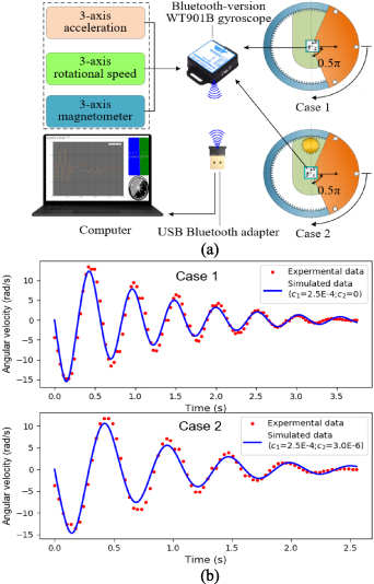
Figure 6. Estimation of damping coefficients: (a) experimental setup; (b) comparisons between the experimental and simulated angular velocity.
Download figure:
Standard image High-resolution image5.3. The recovery torque and potential energy of the VEH
Although equation (3) allows a fast calculation of the magnetic force, simplifying magnets to magnetic dipoles without considering their sizes may lead to considerable errors. Thus, this study also investigates the influence of magnet distance  (the distance between centres of the fixed and tip magnets when the angular position
  is 0) on the accuracy of equation (3) for the magnetic force through comparisons with experimental data. Figure 7(a) presents the experimental setup to measure the magnetic force-induced recovery torque. The VEH is horizontally fixed on a tabletop for eliminating the interference by gravity. The tip of a digital torque screwdriver is put into the head of a screw fixed on the centre of rotation of the pendulum-flywheel structure to measure the torques at different angular positions. The digital screwdriver employed in this experiment has a measuring range of 0–0.5
  and a resolution of 0.0001
  . The magnet distance
  is set to 20 mm, 25 mm, 30 mm, and 35 mm in experiments, respectively.
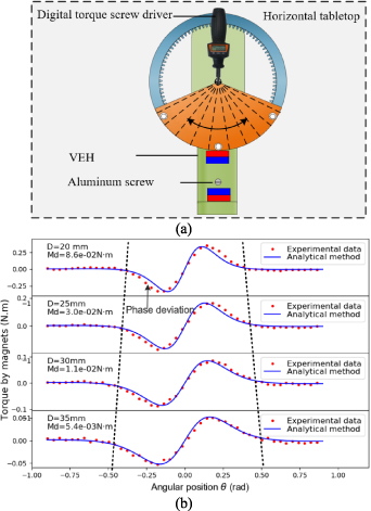
Figure 7. Comparison between the experimental and analytical recovery torques by magnets: (a) experimental setup; (b) comparison results.
Download figure:
Standard image High-resolution imageFigure 7(b) shows the recovery torques obtained by experiments (red points) and analytical calculation (blue lines). The segment of each torque curve between the two black dotted lines in figure 7(b) indicates the angular range of influence of the magnetic force where it becomes large as  increases. However, the magnitude of the recovery torque drops sharply with the increase of
  . There is also a slight phase deviation between the experimental and calculated data when the two magnets are close because of the size effect of magnets. The maximum deviation between the experimental and calculated data decreases from 8.6E-2
 to 5.4 × 10⁻³
 when distance
  increases from 20 mm to 35 mm. For ensuring the precision of calculated results, we suggest that
  should not be less than 20 mm.
The recovery torque of the system can be expressed as  . By integrating
  from angle
  to
to  , the potential energy of the system can be obtained. Figure 8(a) describes the recovery torques of the system induced by gravity and magnetic repulsion at the magnet distance of 20 mm, 25 mm, 30 mm, 35 mm, and 'INF' ('INF' denotes infinite magnet distance), respectively. We can conclude from the figure that magnetic forces influence the recovery torque of the system within an angular range from −0.5 rad to 0.5 rad, but gravity in the range -
 rad to
  rad. However, the magnitude of the recovery torque varies sharply within the angular range of influence of the magnetic force. Introducing the magnetic force to the harvesting system can significantly increase the system's nonlinearity. Gravity and the magnetic force work together to generate a double-well potential energy structure, as shown in figure 8(b). The wells of the potential energy become deep as distance
  decreases. Under the pendulum mode, this system oscillates within one well or jumps between the two wells. However, under the flywheel mode, the system rotates around the centre of rotation, namely, continuously escaping from one cycle and entering another.
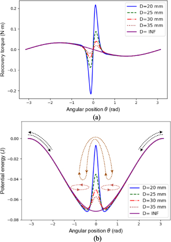
Figure 8. The recovery torques and potential energies of the VEH: (a) the recovery torques of the system; (b) the potential energies of the system.
Download figure:
Standard image High-resolution image5.4. Estimation of the optimal resistance of the external load
During energy generation, the DC generator and the electrical load need to be connected to the same circuit, as shown in figure 3(b). For obtaining higher energy harvesting efficiency, the resistance of the electrical load should match with the internal resistance of the DC generator. This study performs a series of simulations based on the established theoretical model to estimate the optimal resistance of the external load. The sinusoidal excitation with an amplitude of 10 mm and a frequency of 5 Hz is employed in all simulations. 'LSODA', a wrapper to the Fortran solver, is used to solve the ODEs of this harvesting system. For each case, the total integration time is set to 10 s and the time step 1 × 10⁻³ s. The root mean square (RMS) values of instantaneous power at the magnet distance of 20 mm, 25 mm, 30 mm, and 'INF' are calculated to evaluate the harvested energy [50]. Figure 9 presents the simulation results when the resistance of the external load varies from 0 to 200  . The black dashed line indicates the locations of the maximum average power. The results demonstrate that the VEH can obtain its maximum output when the resistance of the external load equals to that of the DC generator. This figure also indicates that decreasing
  is conducive to improving energy harvesting efficiency.

Figure 9. The optimal resistance of the external load.
Download figure:
Standard image High-resolution image6. Numerical analysis of the VEH's dynamical behaviours
The introduction of the magnetic force strengthens the nonlinear characteristics of the VEH, enriching the system's dynamical behaviours. Not only intra-well oscillations with small angular amplitude but also inter-well oscillations in a broad angular range, even continuous rotations, occur during its operations. The nonlinearity of the system increases with angular motions, and strong nonlinearity will make it impossible to obtain any analytical solution of equation (5). In this work, 'LSODA' solver, a numerical method, is used to solve the ordinary differential equations (ODEs) of this dynamical system. This algorithm can switch automatically between the backward difference (BDF) method and the Adams method utilising the numerical information at the end of each time step during the integration [51]. The BDF is one of the linear multistep methods for solving stiff differential equations [52]. The Adams method is more suitable for nonstiff systems [51]. Being able to automatically switch to the proper method makes the 'LSODA' scheme more efficient, especially for complex dynamic systems.
This study carries out a series of numerical simulations to better understand the dynamical characteristics of this energy harvesting system. The typical phase trajectories of different motion modes, frequency response characteristics, the influence factors on the basins of attractions, and the influence factors on the transition from the pendulum mode to the flywheel one are discussed in the simulated studies. The parameters estimated in section 5.1 are employed. During simulations, the time step is always fixed at 1 × 10⁻³ s.
6.1. Typical trajectories of different motion modes
This VEH system has two distinct motion modes: the pendulum and flywheel modes. Figures 10(a) and (b) displaythe typical phase trajectories and time histories of the pendulum mode. The two circles with star and circle makers in figure 10(a) are the phase trajectories of intra-well oscillations under the sinusoidal excitation (amplitude of displacement: 5 mm; frequency: 3 Hz). All the parameters of the two intra-well oscillations are set the same, but the initial position  (left circle: corresponding to the left stable equilibrium point of −0.40
  ; right circle: corresponding to the right stable point of 0.40
  ). The blue line with triangle markers in figure 10(a) refers to the phase trajectory of inter-well oscillation. Compared with the intra-well oscillations, the excitation amplitude increases from 5 mm to 30 mm. The green line with square markers in figure 10(a) is the phase trajectory corresponding to the situation of removing the fixed magnet from the harvester and employing the same 30 mm-amplitude excitations. The comparison between the trajectories before and after removing the fixed magnets indicates that introducing the magnetic force enables the VEH system to have a multi-stable motion, as well as larger oscillation amplitude and velocity. As for the pendulum mode, the inter-well oscillation has a larger response amplitude and velocity than intra-well oscillation, which means that more kinetic energy can be converted into electricity.

Figure 10. Typical phase trajectories and time histories of different movement motes: (a) the phase trajectories of pendulum-motion mode; (b) the time histories of pendulum-motion mode; (c) the phase trajectory of flywheel-motion mode; (d) the time history of flywheel-motion mode.
Download figure:
Standard image High-resolution imageFigures 10(c) and (d) show the phase trajectory and time history of the angular motion in the flywheel mode under the sinusoidal excitation (amplitude: 20 mm; frequency: 7.5 Hz). Under certain conditions, the system can rotate continuously like a flywheel, as shown in figure 10(c) and (d). Comparisons between figures 10(a) and (c) indicate that the maximum angular speed under the flywheel-mode is larger than that in the pendulum mode, causing more kinetic energy to be converted into electricity.
6.2. Frequency-response characteristics of the harvesting system
Introducing nonlinearity to energy harvesting systems is beneficial in broadening the band of response frequencies. This study conducts linear frequency-sweeping simulations to investigate the frequency-response characteristics of the proposed VEH. During linear frequency sweepings, excitation amplitude  remains constant, and excitation frequency
  increases linearly, which can be expressed as a function of time
  :
:
where  is the initial frequency;
  denotes the final frequency;
  stands for the time it takes to sweep from
  to
to  .
.
The switch between the pendulum and flywheel modes mainly depends on external excitations. Generally, the pendulum mode corresponds to weak excitations, while the flywheel mode to the large excitations. To investigate the influence of distance  on the dynamical responses and avoid the interference from the transition of motion modes, we perform frequency-sweeping simulations with small excitation amplitudes of 2 mm, 4 mm, and 8 mm. Under weak excitations, the VEH always stays in the pendulum mode, allowing us to assess the influence of distance
  .
.
For comparison, the angular displacement relative to the stable equilibrium point where the harvester initially stays is used to describe the dynamical response of this VEH. Figure 11 presents the angular displacement of the harvesting system at the magnet distances of 20 mm, 25 mm, 30 mm, 35 mm, and 'INF'. Figures 11(a) and (b) depict the angular displacements of forward and backward frequency-sweeping simulations.

Figure 11. Frequency responses of angular displacement under different excitations: (a) forward sweep; (b) backward sweep.
Download figure:
Standard image High-resolution imageFor the forward sweep, the excitation frequency linearly increases from 0 Hz to 20 Hz in 200 s and decreases from 20 Hz to 0 Hz for the backward sweep. Figure 11(a) shows that the first resonant peak occurs within the frequency range from 1 Hz to 5 Hz. The peak value of the first resonant peak grows with the decrease of the distance  , and the corresponding central frequency increases as well. According to equation (16) the natural frequencies of this system at different magnet distances are estimated: 20 mm: 4.97 Hz; 25 mm: 4.13 Hz; 30 mm: 3.60 Hz; 35 mm: 3.17 Hz; 'INF': 1.57 Hz. The estimated results show a good consistency with the central frequency of first resonant peaks at different magnet distances, indicating the correctness of equation (16). In the middle and lower subplots of figure 11(a), the second resonant peaks appear in the frequency range from 6.0 Hz to 13 Hz when the magnet distance
  equals to 20 mm and 25 mm. The height of the second resonant peaks increases with the excitation amplitude but drops off when the magnet distance
  becomes larger. The above results indicate that decreasing the magnetic force and increasing excitation displacements are conducive to increasing the amplitude of dynamical responses. Moreover, the smaller the distance
  is, the more easily it is to cause the second resonant peak, broadening the response-frequency band. Compared with the result of forward sweep in figure 11(a), the second resonant peaks tend to move to low frequencies, as shown in figure 11(b).
The motion modes of the VEH change with base excitation, especially when excitation magnitude varies dramatically. Nonlinear dynamic behaviours, such as chaos and bifurcations, often occur when the VEH is subjected to intense excitations. This study carries out linear frequency-sweeping simulations to investigate the influence of nonlinear dynamic behaviours on energy harvesting efficiency. During simulations, the excitation amplitude is fixed at 20 mm while frequency sweeping from 0 to 20 Hz takes 200 s.
For a sinusoidal excitation with a constant frequency  , the point set of Poincaré sections,
  , can be extracted from time series
  (
( denotes the total number of signal points), as given in

As the base excitation is sinusoidal and periodic,  , the number of points in one period of excitation, can be represented as
  , where
  is the time step in the numerical integration.
  is also the period to resample the points of a Poincaré section;
  can be any integer within the range of
  1,
1,![${\text{ }}n]$](https://content.cld.iop.org/journals/0964-1726/29/11/115023/revision3/smsabacafieqn183.gif) . Thus, we can extract the k-th point in each period of excitation to form the series
. Thus, we can extract the k-th point in each period of excitation to form the series  ;
;  denotes the size of
  , namely the total number of periods of excitation contained in the time series
  , satisfying
  . However, as for linear frequency sweeping, the excitation frequency
  is a function of time
  expressed by equation (18). Therefore, the sampling period
  is time-varying and can be rewritten as follows:
Currently,  should be a positive integer smaller than
  .
.
By using the above algorithm, the results of linear frequency sweeping are shown in figure 12. Figures 12(a)–(c) correspond to the results with the magnet distance of 'INF,' 30 mm, and 20 mm. The cyan lines denote time series of angular displacement, angular velocity, and instantaneous power, and the black dots overlaid onto the time-series data are the stroboscopic sampling points (points of Poincaré sections). The time series shows the angular displacement and velocity of the pendulum-flywheel structure at a given frequency. The stroboscopic points show the periodicity of the responses concerning excitation frequency.

Figure 12. Bifurcation diagrams and power spectrum density (PSD) curves of the responses of the harvesting system: (a) Bifurcation diagram when  ; (b) Bifurcation diagram when
  30 mm; (c) Bifurcation diagram when
  20 mm; (d) PSD curves of angular velocity.
Download figure:
Standard image High-resolution imageWhen  =INF, the VEH always stays in a periodical motion state with an increase of excitation frequency. The angular velocity and instantaneous power reach their maximum values at the frequency of 11.5 Hz. When
 =30 mm, the dynamic behaviour becomes more complicated; chaotic, quasi-periodic, and periodical oscillations occur and switch between them, as shown in the upper subplot of bifurcation in figure 12(b). The VEH goes through a series of mode transitions: intra-well oscillation (periodic)→ inter-well oscillation (chaotic)→ intra-well oscillation (periodic)→ inter-well oscillation (chaotic)→ inter-well oscillation (quasi-periodic)→ intra-well oscillation (periodic). As shown by the lower subplot of figure 12(b), the instantaneous power reaches larger values within the frequency range from 2.5 Hz to 7.5 Hz, especially during the chaotic oscillation. When
  =20 mm, both pendulum oscillation and flywheel rotation appear during frequency sweeping, as shown in figure 12(c). The middle subplot of figure 12(c) shows that the VEH system experiences intra-well oscillation (periodic), flywheel rotation (chaotic), inter-well oscillation (chaotic), flywheel rotation (chaotic), and intra-well oscillation (periodic) in turn. The VEH system has a higher instantaneous power from 4 Hz to 11 Hz. Comparisons among the instantaneous powers in figures 12(a)–(c) illustrate that the maximum instantaneous power increases when reducing magnet distance, that is, energy harvesting efficiency can be promoted by reducing the magnet distance. Figure 12(d) presents the power spectral density (PSD) curves of angular velocity at magnet distances of 'INF', 30 mm, and 20 mm. The PSD curves become rougher and have larger values when reducing magnet distance, especially in the low-frequency range.
The above analyses indicate that reducing magnet distance can increase the nonlinearity of the VEH system, causing nonlinear dynamic behaviours, such as chaos and bifurcation. Compared with intra-well oscillation, nonlinear dynamic behaviours, including chaotic oscillation, inter-well oscillation, and flywheel rotation, have larger energy outputs. Therefore, we can control the nonlinearity of the system by adjusting magnet distance for improving energy harvesting efficiency.
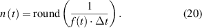
6.3. The influence factors on the basins of attractions
Besides the magnet distance and base excitation, initial conditions of the system also have significant influences on the dynamical behaviours of the harvester. Calculating the basins of attractions of high energy orbits helps understand the system's dynamic characteristics. Figure 13 shows the basins of attractions of six cases: Case 1:  =0 mm,
  =0 Hz,
  =30 mm; Case 2:
  = 10 mm;
 =5 Hz;
  =30 mm; Case 3:
  =10 mm,
  =7.5 Hz;
  =30 mm; Case 4:
 =20 mm,
  =7.5 Hz,
  =30 mm; Case 5:
  =20 mm,
  =7.5 Hz,
 =25 mm; Case 6:
  =20 mm,
  =7.5 Hz,
 =30 mm (
 : the amplitude of sinusoidal excitations;
  : the frequency of sinusoidal excitations). Each figure is made by initialising initial conditions on a rectangular grid. Then, each initial condition is integrated forward to see which attractor its orbit finally approaches. If the orbit approaches the left attractor, a blue dot is drawn on the grid, and if the right one, a red dot is plotted. However, if the orbit remains a hunting oscillation between the two attractors, no dot is plotted.
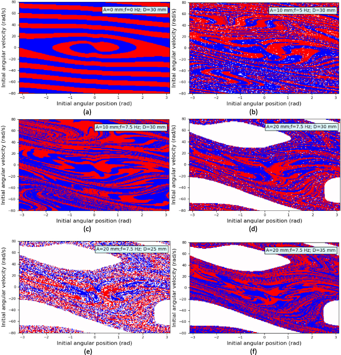
Figure 13. Basins of attractions of this pendulum-flywheel harvester: (a): Case 1; (b) Case 2; (c) Case 3; (d) Case 4; (e) Case 5; (f) Case 6.
Download figure:
Standard image High-resolution imageFigure 13(a) demonstrates that the basins of attractions of the system have distinct boundaries and an anti-symmetry without base excitations. The orbits of all initial conditions eventually come to rest at the left or right attractors in Case 1. The VEH is subjected to a sinusoidal excitation (amplitude:10 mm; frequency: 5 Hz) in Case 2. The boundaries of basins of attractions of Case 2 now display a fractal structure, which indicates that external excitations can make the system more sensitive to initial conditions. Besides, the anti-symmetry of the system also disappears after applying external excitations. Based on Case 2, the excitation frequency of Case 3 increases from 5 Hz to 7.5 Hz, and the excitation amplitude of Case 4 has a further increase from 10 mm to 20 mm. The comparisons among Case 2, Case 3, and Case 4 reveal that both the frequency and amplitude of excitations have influences on the topology of the basins of attractions. Case 4, Case 5, and Case 6 share the same sinusoidal excitation but different magnet distances. It can be seen from figures 13(d)–(f) that the closer the magnets are, the more complicated the topology of the basins of attractions. The above analyses show that both excitations and magnet distance can change the sensitivity of the system to initial conditions.
6.4. The influence factors on the conversion from pendulum mode to flywheel mode
One of the crucial differences between the pendulum and flywheel modes is energy conversion efficiency. Generally, the VEH system in the flywheel mode can harvest more energy than that in the pendulum mode. Therefore, this study investigates the influence factors on the occurrence of flywheel rotation. Figure 14(a) is made by dividing the amplitude and frequency of excitations into a rectangular grid. The motion trajectory under each excitation is integrated to see which motion modes the VEH system takes. If flywheel rotation occurs during integration, a mark (blue square:  =20 mm; red circle:
 =30 mm; black dot:
  =INF) is plotted on the grid. The overlapped area of the blue squares, red circles, and black points in the upper right corner of figure 14(a) indicates when the amplitude and frequency of excitation are large enough, the flywheel motion mode occurs regardless of the absence or presence of the magnetic force. However, numerous blue squares appear within the frequency range of 5–15 Hz in figure 14(a), indicating that the magnetic force is helpful to cause flywheel motions even at small displacements and low frequencies. Figure 14(b) shows the comparison between the situations with or without the magnetic force. The VEH system is subjected to the same sinusoidal excitation (amplitude: 20.4 mm; frequency: 9.2 Hz) under the two situations. The upper subplot of figure 14(b) shows that flywheel rotation occurs when the magnetic force exists, and this system remains in pendulum oscillation after removing the fixed magnet. Furthermore, the instantaneous power of the system in the flywheel mode is higher than that in the pendulum mode.

Figure 14. Influence factors on the conversion of motion modes: (a) conditions for the occurrence of flywheel rotation; (b) the typical comparison between the pendulum and flywheel modes.
Download figure:
Standard image High-resolution image7. Experimental verification of the theoretical model
The shake table (DC3200-36, by Suzhou Sushi Testing Instrument Co., Ltd.) utilised in experiments has an operating frequency range of 5–2000 Hz and a maximum horizontal displacement of 20 mm. During tests, the frame of the harvester is mounted on the horizontal table by bolts. Bluetooth-version gyroscope is stuck as an accessory on the fan-shaped pendulum. Angular velocity of the pendulum structure is recorded at a sampling frequency of 200 Hz and transmitted to the computer in real-time via Bluetooth. The DC generator and an electrical load with the same resistance are connected to a closed circuit. The voltage across the electrical load is recorded with an oscilloscope (TPS2000, by Tektronix, Inc) at a sampling frequency of 5000 Hz. The experimental setup is shown in figure 15(a).
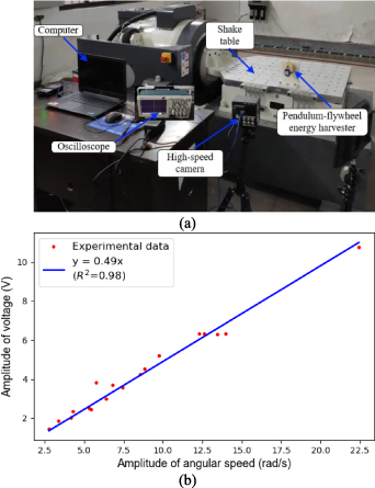
Figure 15. Experimental verification of the theoretical model: (a) experimental setup; (b) relationship between the angular velocity and electromotive voltage.
Download figure:
Standard image High-resolution imageOur simulations suggest that the VEH system has large dynamical responses within the frequency range of 3–13 Hz. Considering the performance of the shake table, the frequencies of 5 Hz,7.5 Hz, and 10 Hz are taken in the experiments. The excitation amplitudes are set to 10 mm and 15 mm, and the magnet distance at 20 mm, 30 mm, and 40 mm, respectively. There are a total of 18 cases designed in experiments (excitation frequency: 5 Hz, 7.5 Hz, and 10 Hz; excitation amplitude: 10 mm and 15 mm; magnet distance: 20 mm, 30 mm, and 40 mm; cases). First, the experimental data is used to verify the relationship between the electromotive force of the generator and the angular velocity of the pendulum. Then, the experimental and simulated angular velocities of the pendulum structure are analysed.
The induced electromotive voltage  by the generator is assumed to be proportional to the angular velocity
  of the pendulum. Part of the tests is to verify the linear relationship between the two variables. The electromotive voltage of the generator can be calculated according to the measured voltage across the electrical load. Eighteen points in figure 15(b) are plotted according to the amplitudes of angular velocity and the electromotive voltage in those 18 cases. The blue line represents the best fitting results using the least-square method. The coefficient of determination (
 ) reaches 0.98, indicating that there is a good linear relationship between the induced electromotive voltage and the angular velocity of the pendulum. The slope of the fitting line is 0.49, whereas the theoretical value is 0.53, meaning a relative error of 7.5%.
This study also compares the experimental and simulated angular velocities of the pendulum structure for validating the theoretical model. Table 2 shows the comparison results of the amplitudes of angular velocity under different cases. One can see from the table that the amplitude of angular velocity decreases with the increase of the magnet distance. The relative errors of most cases are less than 10% when the amplitude is 10 mm, and these increase when the amplitude increase to 15 mm. Nevertheless, sometimes more significant errors may occur in some instances, and the maximum relative error reaches 38%.
Table 2. The comparison between the experimental and simulated angular velocity.
 =10 mm =10 mm |
 = 15 mm = 15 mm | ||||||||
|---|---|---|---|---|---|---|---|---|---|
| (mm) | (HZ) | Simulated (rad s−1) | Experimental (rad s−1) | Error rate | Experimental Power (RMS, mW) | Simulated (rad s−1) | Experimental (rad s−1) | Error rate | Experimental Power (RMS, mW) |
 = 20 = 20 | f = 5 | 4.8 | 5.2 | 7.6% | 5.3 | 7.2 | 6.4 | 12.5% | 7.9 |
| f = 7.5 | 10.0 | 10.2 | 2.0% | 13.6 | 14.1 | 11.8 | 19.5% | 15.8 | |
| f = 10 | 7.3 | 7.0 | 4.2% | 8.7 | 21.0 | 22.4 | 6.3% | 16.3 | |
 = 30 = 30 | f = 5 | 3.5 | 3.8 | 7.9% | 3.5 | 6.5 | 5.3 | 22.6% | 5.5 |
| f = 7.5 | 3.7 | 6.0 | 38.3% | 5.6 | 5.4 | 7.7 | 29.9% | 7.5 | |
| f = 10 | 4.6 | 4.7 | 3.3% | 7.4 | 6.7 | 5.0 | 34.0% | 7.3 | |
 = 40 = 40 | f = 5 | 2.7 | 2.7 | 0 | 2.5 | 3.9 | 4.1 | 4.9% | 4.2 |
| f = 7.5 | 3.5 | 3.3 | 6.0% | 3.9 | 5.2 | 5.1 | 2.0% | 7.3 | |
| f = 10 | 4.6 | 4.2 | 9.5% | 7.0 | 6.7 | 5.7 | 17.5% | 10.6 | |
The errors may originate from the following sources:
(1) Modelling errors. In establishing the theoretical model, the magnets are simplified as dipole moments; the components of the harvester are simplified as uniform-rigid bodies; the mechanical damping force is assumed to be proportional to the angular velocity of the system; Assuming this VEH usually works at low frequencies, the inductance of the DC generator is not considered. These simplifications should lead to errors.
(2) Manufacturing and assembly errors. Errors may occur during the process of fabricating these components and assembling the harvester. These factors have influences on the dynamical behaviours of the system.
(3) Disturbance from the shake table. During operation, the power supply to the shake table can generate a small but noticeable amount of unwanted vibration to the shake table, consequently providing additional small excitation to the VEH. This disturbance would increase with the amplitude of excitation.
(4) Measurement errors. Because of the limitation of sensors and interference from the environment, there inherent errors in the measured results.
(5) The nonlinearity of the system. The system becomes more sensitive to the initial conditions of the system with the increase of nonlinearity, which explains why the errors increase with excitation amplitudes.
The RMS values of the instantaneous power in different experimental cases are calculated and presented in table 2. It is clear from the table that this VEH reaches its maximum energy output of 16.3 mW at the magnet distance of 20 mm when subjected to excitation with an amplitude of 15 mm and a frequency of 10 Hz. In order to report the agreement between the experimental and simulation data, the results of two typical cases are presented in figure 16. The results under a small excitation (amplitude: 10 mm; frequency: 5 Hz;  = 30 mm) are presented in figure 16(a). Figure 16(b) corresponds to the results of an intense excitation (amplitude: 15 mm; frequency: 10 Hz;
  = 20 mm). The results indicate that the experimental data is in good agreement with the simulation data when the excitation is small. However, the amplitude of the dynamical response has a slight difference when the excitation is large. On the whole, the experimental and simulation data have similar waveforms, as shown in figure 16(c). We also compare this harvester with some other state-of-the-art pendulum-based VEHs, as shown in table 3, and the proposed pendulum-flywheel VEH is found to exhibit good performance in relation to piezoelectric and electromagnetic VEHs. However, it should be pointed out that the comparisons should be treated with care since other parameters such as the size and mass of the VEHs can be different, which influence the energy harvesting performance.

Figure 16. Comparison between the simulated and experimental time-history data: (a) results under a small excitation; (b) results under a large excitation; (3) enlarged view of the waveforms in the black dashed wireframes.
Download figure:
Standard image High-resolution image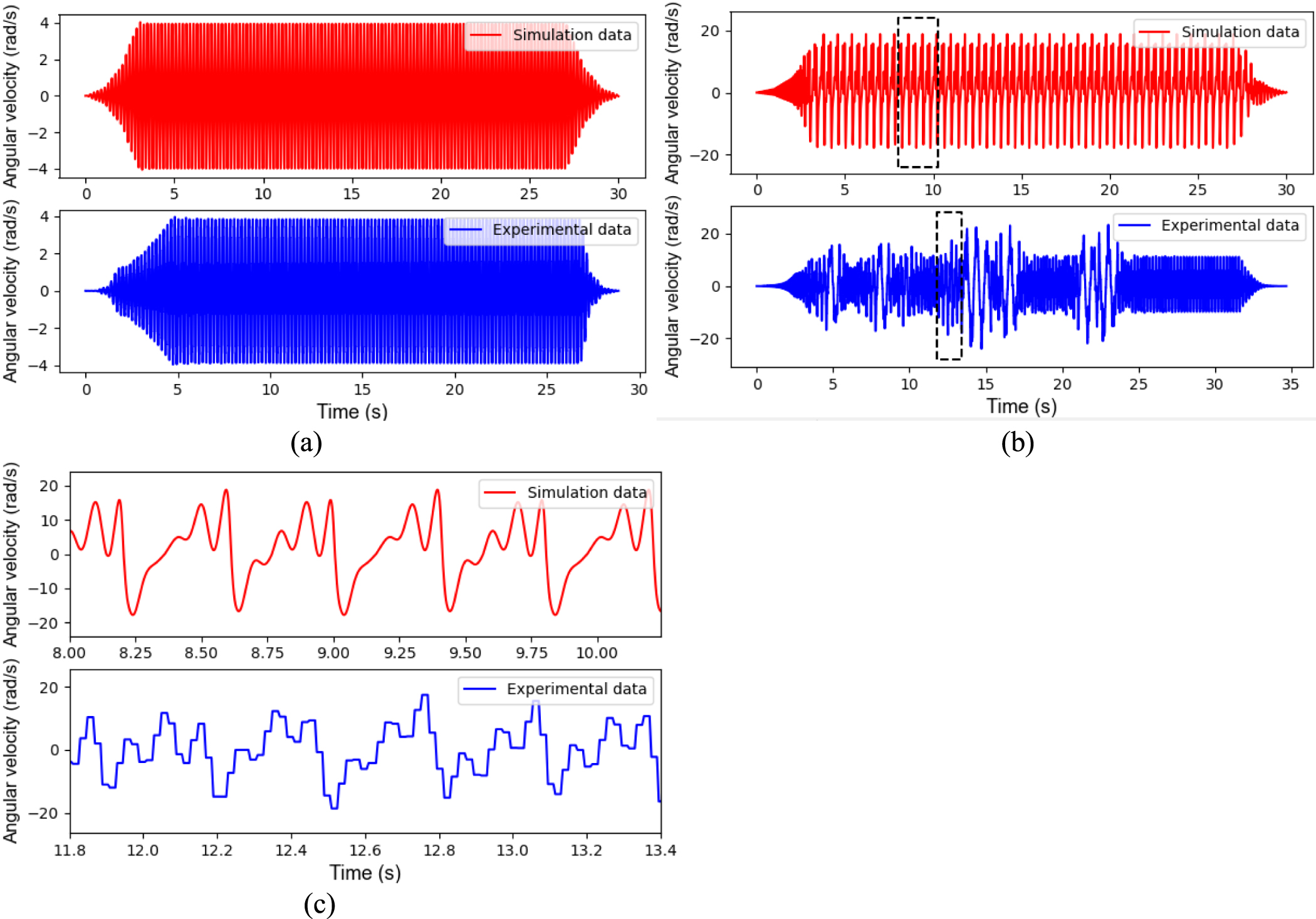
Table 3. Comparison with the state-of-art pendulum-based VEHs.
| Authors/year/reference | Structural feature | Transducer | Maximum size | Excitation acceleration/amplitude | Excitation frequency | Maximum power |
|---|---|---|---|---|---|---|
| This work | Pendulum- flywheel | Electromagnetic | 154 mm | 15 mm | 10 Hz | 16.3 mW |
| Kuang et al/2019/[53] | Magnetic rolling pendulum | Electromagnetic | 50 mm | 0.5 g | 4 Hz | 3.6 mW |
| Simeone et al/2019/[49] | Single pendulum | Electromagnetic | 176 mm | 197 mm | 7.5 Hz | 120 mW |
| Izadgoshasb et al/2019/[8] | Cantilever beam-double pendulum | Piezoelectric | 180 mm | 1 g | 2 Hz | 2 mW |
| Kumar et al/2019/[32] | Double pendulum | Electromagnetic | 140 mm | 15 mm | 7.9 Hz | 0.68 mW |
| Malaji et al/2018/[14] | Two mechanically coupled pendulums | Electromagnetic | 60 mm | 2.3 mm | 2.5 Hz | 0.25 mW |
| Wu et al/2018/[1] | Spring pendulum | Piezoelectric | 112 mm | 0.05 g | 1.83 | 13.29 mW |
8. Conclusion
In this work, we propose a pendulum-flywheel device for harvesting vibration energy. This VEH has two work modes: the pendulum mode corresponding to weak base excitations and flywheel mode corresponding to intense excitations, which enable the harvester has strong adaptability to various excitations in nature. Magnetic force, generating a bistable potential well, is introduced to the system for increasing the system's nonlinearity and broadening its frequency band.
The simulation results indicate that reducing magnet distance can significantly enhance the system's nonlinearity, enlarging the amplitude of dynamic responses and broadening its frequency band. The results also show that the magnet distance influences the switch of the VEH's motion modes. This characteristic provides us with an approach to control the performance of the harvester for adapting to different excitations. Besides, experiments are performed to verify the reasonability of the theoretical model. The experimental data verify the linear relationship between the induced electromotive voltage and the angular velocity of the pendulum structure with a coefficient of determination ( ) of 0.98 and a slop error rate of 7.5%. The angular velocity of the system obtained by simulations agrees well with the experimental data when the excitation displacement is small (the error rate of most cases is less than 10%). However, the error rate has an increase with the amplitude because the nonlinearity of the system increases with the swing angle of the pendulum and makes the system more sensitive to the initial conditions. In experiments, this VEH reaches its maximum energy output of 16.3 mW, which exhibits good performance in comparison with state-of-art pendulum-based VEHs.
Next, we intend to investigate the influences of random excitation on the performance of the harvester and try to optimise its geometry. During establishing the theoretical model, a series of simplifications are made. In a further study, we plan to investigate how these simplifications influence the fidelity of the theoretical model and improve it. Besides, we would also like to use the proposed harvester to establish a self-powered sensor node for condition monitoring of freight trains and test its performance in real scenery.
Acknowledgments
The main theoretical work is conducted by the first author during his visit to the University of Liverpool under the supervision of the 3rd author and sponsored by China Scholarship Council. This research is also funded by the National Natural Science Foundation of China, Grant Nos. 51878576 and U1934214.