

Abstract
Periodic structures are growing in popularity especially in the energy harvesting and metastructures communities. Common types of these unique structures are referred to in the literature as zigzag, orthogonal spiral, fan-folded, and longitudinal zigzag structures. Many of these studies on periodic structures have two competing goals in common: (a) minimizing natural frequency, and (b) minimizing mass or volume. These goals suggest that no single design is best for all applications; therefore, there is a need for design optimization and comparison tools which first require efficient easy-to-implement models. All available structural dynamics models for these types of structures do provide exact analytical solutions; however, they are complex requiring tedious implementation and providing more information than necessary for practical applications making them computationally inefficient. This paper presents experimentally validated recursive models that are able to very accurately and efficiently predict the dynamics of the four most common types of periodic structures. The proposed modeling technique employs a combination of static deflection formulae and Rayleigh's Quotient to estimate the first mode shape and natural frequency of periodic structures having any number of beams. Also included in this paper are the results of an extensive experimental validation study which show excellent agreement between model prediction and measurement. Lastly, the proposed models are used to evaluate the performance of each type of structure. Results of this performance evaluation reveal key advantages and disadvantages associated with each type of structure.
Export citation and abstract BibTeX RIS
1. Introduction
Periodic structures are gaining popularity in the structural dynamics community. More specifically, recent periodic structure modeling efforts are being made in research related to energy harvesting and metastructures. The primary motivation driving a majority of these efforts is the ability of these unique structures to have low natural frequencies and compact geometries. One can quickly see that minimizing the size and the natural frequency of a structure are competing objectives. For example: the natural frequency of a simple cantilever beam is inversely proportional to the square of its length i.e.,  Reducing the natural frequency by simply reducing thickness or adding a tip mass to the cantilever causes excessive stress which quickly exceeds allowable limits. In an attempt to address this fundamental scaling problem, researchers have proposed several types of structures that have repeating geometries. These unique structures are essentially comprised of a series of beams attached in some cycle or pattern and are therefore referred to here as periodic structures.
Among the first to propose periodic structures for energy harvesting were Karami and Inman (2009) where a zigzag type geometry was shown to significantly reduce natural frequency in a compact design while maintaining relatively low stress levels [1]. This simple yet effective design was later the subject of several works by Karami et al in energy harvesting including energy harvesting from heartbeat vibration for powering pacemakers [2–4]. The zigzag structure has also been used for nonlinear energy harvesting by Essink et al (2015) where a recursive formula was used to estimate the natural frequency and mode shape of the first mode of vibration [5]. Here, the authors were able to show through experimental validation that the recursive model could be used to very accurately predict the power produced from harmonic base excitation of a zigzag structure having a piezoelectric layer. At the same time, Hobeck and Inman (2015) showed that a network of zigzag structures integrated into a host structure (called a metastructure) could be used as a distributed passive vibration mitigation system [6]. Here, Hobeck and Inman proposed and validated a general Rayleigh–Ritz model for a cantilevered metastructure and also presented the first nonlinear metastructure where opposing magnets were used to induce internal nonlinearities which greatly enhanced the vibration suppression performance. Very recently this exact structure was the subject of a study performed by Abdeljaber et al [7] where the authors implemented a genetic algorithm optimization scheme using the model proposed by Hobeck and Inman in [6].
Another type of periodic structure discussed in the literature includes orthogonal spiral (OS) structures—also referred to as spiral cantilevers. An OS energy harvester was proposed by Bai et al (2014) where magnets were used to induce nonlinearities which were shown to enhance the energy harvesting performance [8]. More recently Santos et al (2016) presented a complete analysis on a distributed parameter analytical model for OS structures [9].
The final type of popular periodic structure discussed in the literature is that of the stacked zigzag (SZ) structure—also called the folded-back beam, the fan-folded structure, or the flexible longitudinal zigzag structure. Initially interested in repeated resonances in these unique structures, Khattak et al was among the first to propose a model for the SZ [10]. Recently, Ansari and Karami (2016) used this type of structure for harvesting energy from heartbeat vibration where they presented an experimentally validated fully coupled analytical electromechanical model [11]. A similar structure and model presented by Zhou et al (2016) focused on energy harvesting from harmonic base excitation [12]. The most recent related research by Zhou et al (2017) demonstrated how effective longitudinal zigzag structures are at harvesting energy when the base excitation is applied at various angles [13].
A general model for energy harvesting from a structure with geometric discontinuities was recently proposed by Wickenheiser [14]. His along with most models developed for periodic structures are analytical distributed parameter continuous system type models which are formulated by first treating each beam segment as a Euler–Bernoulli (EB) beam. Local mode shapes are then assumed which requires enforcing proper boundary and continuity conditions on both ends of each beam segment and tediously deriving lengthy orthogonality conditions. The system of equations is eventually arranged into matrix form before solving the structural eigenvalue problem using a computational root finding method. Finally, results of the eigenvalue solution provide the natural frequencies, but the mode shapes must then be constructed using the eigenvectors [2–4, 8–12, 15].
The two primary advantages that these existing analytical models have over the proposed recursive numerical models are: first, they provide exact analytical solutions for natural frequency and mode shape. Second, they provide natural frequency and mode shape solutions for higher modes where the proposed models only provide solutions for the first mode. This first-mode limitation should not diminish the value of the proposed models because many applications (especially for energy harvesting) are only interested in the first mode. Furthermore, a primary motivation behind many periodic structure designs is to attain the lowest possible natural frequency; therefore, higher modes are of lesser importance and may be a waste of computational effort.
As previously mentioned, existing dynamics models for periodic structures are fairly complex and may provide more information than necessary for practical applications. Therefore, a major goal of the current research is to provide an efficient means of both implementing and executing the calculations for estimating the first mode dynamics of periodic structures. Unless specified otherwise, all calculations presented in this paper were scripted in MATLAB and executed on a generic laptop with a processor speed of 2.5 GHz and 8 GB of memory. Using this computer system, the natural frequency and mode shape for a zigzag structure with 21 beam segments for example could be calculated in 12.7 ms which is equivalent to executing 78.5 design iterations per second. This computational efficiency makes rapid design optimization readily available which will be the focus of related future research. A comparison between a proposed model and commercial finite element analysis software will be discussed toward the end of this paper.
The novelty of the models presented in this paper compared to current models is that they are efficient, reduced-order, closed-form models that yield natural frequency predictions with accuracies equal to or greater than existing higher-order analytical and finite element models. The novelty of the proposed modeling approach is that the deflection equations for each beam segment of the periodic structures are predetermined closed-form functions of both body forces and applied loads caused by adjacent beam segments and attached masses. Because the deflection and loads of each beam segment depend only on those of their nearest neighbors, a simple set of recursive relationships can be used to calculate the forces and resulting deflections in the entire structure. The recursive nature of these relationships allows the mode shape estimate to be calculated directly without solving a set of simultaneous equations or the classic structural eigenvalue problem. Given the mode shape and material properties, the resulting natural frequency can be readily determined using Rayleigh's Quotient.
This paper presents an efficient recursive modeling technique for estimating the first mode dynamics of periodic structures. The models shown here are significantly simplified from those originally developed by the authors in [5]. The proposed modeling technique will be demonstrated on four types of periodic structures: planar zigzag (PZ), SZ, and two types of OSs. Results of an experimental validation study are also shown where natural frequency measurements made on several prototypes of each type of structure are compared to model predictions. Lastly, the models are used to evaluate the performance of each type of structure. Results of this performance evaluation reveal key advantages and disadvantages associated with each type of structure.
2. Modeling
This section proposes four modeling techniques used to predict the mode shape and first natural frequency of three basic types of periodic structures. Before discussing details of each model, it is important to first identify all fundamental assumptions that apply to every structure considered in this analysis. First, it is assumed that each beam segment experiences small deflections where nonlinear effects can be neglected, and superposition can be used to determine total deflection from combined loading. All beam segments are assumed to be inextensible so their lengths remain constant even in the presence of axial loading. It is also assumed that each beam has uniform mass and stiffness properties, and is long and thin so shear deformation and rotational inertia are negligible; therefore, EB beam theory applies.
A final key assumption made in this analysis is that the mode shape of each structure can be approximated from its static deflection resulting from a uniform distributed load acting in the direction of positive deflection. Considering a cantilevered EB beam, the exact theoretical mode shapes can be expressed as,
where  is the free length of the beam and the constant
  is defined as,

which is a function of the natural frequency  linear mass density
  Young's modulus
  and the area moment of inertia
  The deflection of a cantilever beam subject to a uniform distributed load is defined as,

where the tilde  denotes an approximation to the exact solution given in equation (1). Upon normalizing the amplitude of both exact and approximate mode shapes, it is possible to compare both solutions and quantify their differences. As shown in figure 1, both mode shapes are nearly identical with a maximum error of 1.47% and an
  value of 0.999 thus validating the use of static deflection to approximate mode shape. It should be clarified that this limited example considers simple loading on only a cantilevered beam; however, as will be shown in the following sections, cantilever beams are the basic building block of every structure discussed in this paper.
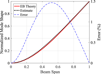
Figure 1. Comparison of exact and approximate first bending mode shape for a cantilever beam.
Download figure:
Standard image High-resolution imageThe general procedure used for defining the mode shape and natural frequency of each structure begins with first defining the local deflection of every beam segment subject to uniform distributed loading. Next, the global deflection (mode shape) of the entire structure is calculated. Lastly, the global deflection is used with Rayleigh's Quotient to calculate the equivalent mass, stiffness, and resulting natural frequency.
2.1. Planar zigzag
The first structural arrangement to be considered is referred to as PZ. Also known in the literature as simply 'zigzag', PZ structures are made up of a series of beams connected in an alternating arrangement. The first beam is fixed at its base while the base of the second beam is attached to the tip of the first, and so on. Each new beam is oriented in the same plane either +90° or −90° relative to the previous beam thus forming the structure illustrated in figure 2.
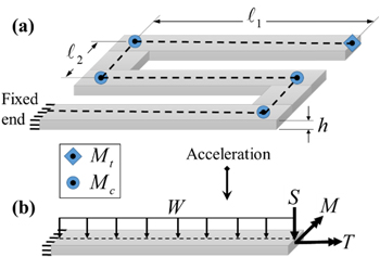
Figure 2. Illustration of planar zigzag structure showing (a) overall design, dimensions, and boundary conditions along with (b) location and direction of each load considered for every beam member.
Download figure:
Standard image High-resolution imageUp to four loads are considered for each beam member, (1) distributed load  caused by beam mass; (2) tip shear load
  from all masses attached to the tip including point masses (
 and
and  ) and previous distributed masses; (3) tip moment
  and (4) tip torque
  The first three loading conditions induce bending deflection
  where positive values of
 and
and  result in positive deflection. The fourth load (torque) is in the axial direction of the beam and results in twisting deflection
  Location and direction of these four forces are shown in figure 2(b).
The effective length of each beam member is approximated by representing the structure as a series of lines rather than beams. This 1D representation is shown in figure 2 as the dashed line. Each line segment travels down the center of each beam and intersects with the centerline of the adjacent beam. Effective beam lengths  and
and  in figure 2 are the lengths of each centerline segment. This effective beam length approximation accounts for 100% of the total mass and for the fact that the connections between beam segments are not rigid.
For this part of the analysis, beam 1 is considered to be the free beam. All loads acting on beam 1 include only shear  due to a point tip mass and distributed load
  due to the beam mass. Given a unit acceleration, the distributed and concentrated loads due to these masses are defined as,


Notice that the distributed load  for each segment is equal to the linear mass density of that segment. Now considering all forces acting on beam 2, we have shear from beam 1 including the weight of beam 1, distributed mass load, and now tip torque
  from the loads acting on beam 1. These loads are defined as,


where  is incremental mass located at each joint and acts as a point tip mass to each beam segment (see figure 2). This incremental mass is used to account for mass that may be added or lost if beams of different thicknesses are joined together.
Continuing with all forces acting on beam segment 3 we have,


where it is now possible to use fundamentals of static beam analysis to define the current shear, moment, and torque as functions of previous forces, geometry, and beam properties. The resulting recursive equations for shear and torque are,


for  where it is no longer necessary to define tip moment
  because it will always be equal to or opposite the torque in the previous beam segment depending on the beam orientation.
With all local forces defined, superposition can be used to determine the bending and torsion deflection of each cantilever beam segment. Beginning with bending given as,
the total local deflection  is found by simply adding the contributions due to shear load, distributed load, and moment respectively, where
  is the length coordinate of the
  beam with values from zero to the length of the
  beam
beam  Recall that beam number 1 is the free beam. The torsional deflection of each beam is defined as,

where  is the torsional stiffness of the
  beam segment which is a function of the shear modulus
  and the torsional constant
  Considering the rectangular cross-section of the beams
  can be defined as,

where  is a function of the ratio of beam thickness
  to width
  and is given as,

Now that all local deflections are known, it is possible to define global deflections for each beam. Except for the fixed beam, continuity conditions require that the global deflection of all beams depends on the global deflection of the beam it is attached to. Enforcing these continuity conditions while defining global deflections requires beginning with the fixed beam deflection which is simply equal to the local deflection given as,

which and has zero slope and deflection at the fixed end. Global deflection of the next beam (beam 2) is defined as,

which is equal to its local deflection; however, the base of this beam has a nonzero displacement and angle which are equal to the tip deflection and twist angle of the first beam. Similar to beam 2, global deflection of beam 3 is given as,
which is equal to its local deflection added to the global tip deflection of beam 2. The base angle of beam 3 is now a function of both the twist angle of beam 2 and the global tip angle of beam 1. Finally, the recursive expression for global displacements can be given as,
for  where the subscript
  denotes the beam segment number beginning with the fixed beam which is opposite of subscript
  used for the local deflections in equations (13) through (16). The final theoretical mode shape determined with equations (19) through (22) for the 5-beam PZ structure shown in figure 2 is given in figure 3 where the shape with dashed lines indicates the neutral position.
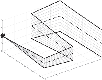
Figure 3. Theoretical first fundamental mode shape of a 5-beam PZ structure (deflection is amplified to emphasize mode shape).
Download figure:
Standard image High-resolution imageGiven the estimated fundamental mode shape defined in equations (19) through (22), Rayleigh's Quotient can be used to determine the equivalent mass, stiffness, and natural frequency of the structure. Rayleigh's Quotient for the PZ structure is defined as,

where  is the natural frequency (rad s−1),
  is the equivalent stiffness,
  is the equivalent mass,
  is the tip displacement of the free beam, and
  is the total number of beam segments. The numerator of equation (23) contains two familiar strain energy terms associated with beam bending and torsion which must be integrated over the length of each beam segment. The denominator of equation (23) has kinetic energy terms that include the mass of each beam segment along with incremental point masses
  at the end of each beam and a tip mass
  at the end of the free bream. This point mass localization is achieved using the Kronecker delta function
  which is equal to one if j = n and is zero otherwise.
2.2. Orthogonal spirals
The second type of periodic structure considered in this analysis is called an OS. Similar to the PZ structures discussed in the previous section, OS structures consist of a series of coplanar beams each attached to the tip of the previous beam as illustrated in figure 4. The difference between PZ and OS designs is that each new beam of the OS structure is oriented 90 degrees relative to the previous but in the same direction i.e., all are at +90° or all are at −90° to form a rectangular spiral.

Figure 4. Illustration of orthogonal spiral structure showing overall design, dimensions, and boundary conditions for (a) outer beam fixed, and (b) center beam fixed along with (c) location and direction of each load considered for every beam member.
Download figure:
Standard image High-resolution imageFollowing a procedure similar to that for the PZ in section 2.1, the individual forces acting on the free beam (beam 1) and beam 2 are identical to those defined in equations (4) through (9). Forces on beam 3 of the OS are defined as,


where the only difference between these and equations (10) through (12) is the sign of previous torque  in the definition of
  The recursive force equations for
  can therefore be defined as,


where the sign of the previous torque  is constant because each beam is attached with the same angle relative to the previous beam unlike the PZ structure. Local bending deflection can be defined as,
and the local torsion deflection as,

where  is the length coordinate of the
  beam with values from zero to the length of the
  beam
beam  and torsional stiffness
  can be defined using equations (17) and (18).
Global deflections for the first three beams of the OS structure (beginning with the fixed beam as beam 1) are equal to equations (19) through (21). The resulting recursive expression for global deflections of the OS can be defined as,
for  where the global index
  denotes beam number where the fixed beam is beam 1 and is opposite the numbering convention of local index
  which starts with the free beam as beam 1. It is important to note that force and deflection equations for the OS structure are reversible depending on the location of the fixed and free beams as long as the index convention is consistent. In other words, the same local and global equations for the OS can be used for either center beam fixed or outer beam fixed as illustrated in figures 4(a), (b). Finally, given the global deflections, Rayleigh's quotient for the OS structure can be defined as,
where the lumped parameter equivalent mass and stiffness are  and
and  respectively. Figure 5 shows the fundamental theoretical mode shapes found using equation (31) for the 7-beam OS structures in figure 4 where the dashed lines indicate the neutral position. Figure 5(a) is for the case of the outer beam fixed while figure 5(b) is for the case of the center beam fixed.

Figure 5. Theoretical first fundamental mode shape of 7-beam OS structures for (a) outer beam fixed, and (b) inner beam fixed (deflection is amplified to emphasize mode shape).
Download figure:
Standard image High-resolution image2.3. Stacked zigzag
The third and final type of periodic structure discussed in this research is called a SZ which is also referred to in the literature as a fan folded structure. Similar to the previously discussed PZ and OS structures, the SZ is a series of attached beams. The first beam is fixed at its base and its tip is attached to the base of the next beam with a rigid joint block. Unlike the coplanar design of the PZ and OS, adjacent beams of the SZ are positioned in orthogonal planes as illustrated in figure 6.
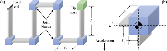
Figure 6. Illustration of stacked zigzag structure showing overall design, dimensions, and boundary conditions for (a) the entire structure, and (b) a detailed view of a joint block.
Download figure:
Standard image High-resolution imageBeginning with the free beam as shown in figure 6, because the uniform loading is acting in the axial direction along the beam, there are no out of plane forces to cause local deflection. This would not be the case however, with an even number of beam segments, so it is necessary to define two sets of recursive equations. Also, notice that unlike the PZ and OS structures, all deflections in the SZ structure are bending only i.e., there is no torsional deflection.
Given an odd number of beam segments, the forces acting on the free beam (beam 1) are,

where tip shear  tip moment
  and distributed force
  are all zero. Forces on beam 2 are defined as,


where all mass of beam 1 along with the tip mass  and joint block mass
  contribute to the tip shear and moment. The tip moment arm
  is the distance from the tip of the second beam to the center of gravity of the block mass which is also the center of gravity of the first beam and tip mass. See figure 6 for reference. Continuing with the analysis, all forces on beam 3 can be expressed as,


where again the tip shear and distributed loads are zero as with beam 1; however, the tip moment is now a function of the previous tip moment  the previous shear
  and the mass of the previous beam. The forces acting on beam 4 are,


which are similar to the forces on beam 2 defined in equations (34) through (36) except that the previous moment  and shear
  are now nonzero and must be accounted for.
Now that all forces can be defined with known constants and previous values, the recursive force equations can be determined. Upon first considering the odd numbered beams for  the forces are,

and the even numbered beam forces  are,
are,


Recall that equations (33) through (46) are for an SZ structure with an odd number of beam segments and oriented as shown in figure 6. Given this same orientation and following a similar procedure for the case of an even number of beam segments one can arrive at an identical set of recursive force equations where the odd and even indices are swapped. In other words, equations (42) and (43) would apply to even numbered beams  and equations (44) through (46) would apply to odd numbered beams
  Forces on the free beam become,


which are the same as those for a simple cantilever with a large tip mass, and the forces on beam 2 are,


The equations for forces on beam 3 are identical to those given in equations (39) through (41) after reducing all indices by 1. Similarly, the equations for forces on beam 4 are identical to those given in equations (37) and (38) after subtracting 1 from every index.
The local deflections for SZ structures can be defined as,
which is similar to equations (15) and (29) with the major difference being that the distributed load  alternates between zero and the linear mass density of the current beam segment. Given all local deflections and geometry, it is possible to determine the global deflections. Beginning with the clamped beam as beam 1, its global deflection is,

which is simply equal to its local deflection. Global deflection of beam 2 can be defined as,

which is equal to the local deflection including the influence of the rotated join block which adds an angle equal to the tip angle of beam 1 and an offset caused by the distance  Global deflection of beam 3 can be expressed as,
which accounts for the joint block angle as with equation (54) but also must include the deflection of the first beam which is in the opposite global direction of beam 3. Continuing with these definitions leads to the recursive set of global deflection equations,
for  where the global index
  begins at 1 for the clamped beam and goes to the number of beam segments
  for the free beam which is in the reverse order of local index
Figure 7 shows the theoretical fundamental mode shape of the 7-beam SZ structure in figure 6 found using equations (53) through (56) where the dashed lines indicate the neutral position. The gaps between corners of each line segment in figure 7 are where the beams are joined by rigid joint blocks. For simplicity and clarity, these blocks were not included in the mode shape plots.
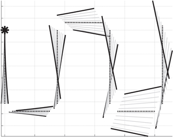
Figure 7. Theoretical first fundamental mode shape of a 7-beam SZ structure (deflection is amplified to emphasize mode shape).
Download figure:
Standard image High-resolution imageAgain, Rayleigh's quotient can be used to define the natural frequency as,
where the equivalent lumped parameter mass and stiffness are  and
and  respectively and the two special functions
  and
and  have been included for convenience. The first function is a mass term defined as,

where the Kronecker delta function  is used to replace the join block mass
  with the tip mass
  on the free beam (for j = N). The second special function is given as,

which is the square of the deflection at the center of mass (defined by  ) attached to the end of the
  beam segment. For simplicity, it is assumed that the center of mass for all join block masses and the tip mass is located at the same distance
  from the end of the beam.
The denominator of Rayleigh's quotient in equation (57) includes three terms beginning with the familiar distributed mass term where the square of the beam deflection must be integrated over the length of each beam segment. The second term is a concentrated mass term associated with the tip deflection of each beam segment. The third and final term in the denominator accounts for in-plane rigid-body-motion of each beam and mass caused by deflection of the previous beam. Of course, the fixed beam does not experience this rigid-body-motion, so the Kronecker delta is used to eliminate the third term for 
3. Experimental validation
Multiple prototypes of the PZ, OS, and SZ structures were fabricated in order to experimentally validate the proposed modeling techniques for predicting natural frequencies. Every test was performed using the following general procedure. First, the structure was clamped to provide the appropriate boundary condition, then measurements were made to ensure the free lengths of each beam segment. Next, the structure was excited using an impulse hammer while measuring the tip velocity of the free beam segment with a laser vibrometer. Tip velocity data was sampled at 250 kHz for 4 s providing an FFT resolution of 0.25 Hz. The natural frequency for each measurement was determined by taking the central frequency of the first prominent peak in the FFT. After recording the measurement, the next structure was mounted and the procedure was repeated.
All prototypes for both PZ and OS type structures were made by using a high-pressure CNC water jet to cut the desired patterns in a sheet of 6061-T6 aluminum. Material properties used in this model validation analysis include a mass density of 2700 kg m−3, Young's modulus of 69 GPa, and Poisson's ratio of 0.3. Overall dimensions of the 21-beam PZ structure were 66.55 mm long and 33.27 mm wide having a uniform thickness of 1.52 mm and a beam segment width of 5.08 mm. Photos of one of the PZ and OS structures is shown in figures 8(a) and (b) respectively. Measurements were made with structures having from 3 to 21 beam segments in 2 beam increments. Results of the PZ measurements are summarized in figure 9 where there is good agreement between model predictions and experimental measurements. The maximum error is 9% for the 3-beam PZ and is less than 2% for all remaining beam numbers.
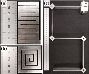
Figure 8. Photos of experimental specimens showing (a) 21-beam PZ, (b) 12-beam OS, and (c) 5-beam SZ structures that were used for part of the model validation process. (A millimeter scale is shown next to each structure.)
Download figure:
Standard image High-resolution image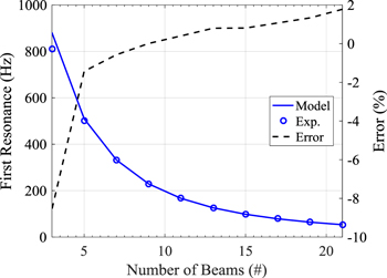
Figure 9. First natural frequencies of a set of PZ structures with 3–21 beams showing error between model prediction and measurement.
Download figure:
Standard image High-resolution imageOverall dimensions of the 12-beam OS structures were 42.16 mm long and 40.00 mm wide having a uniform thickness of 1.52 mm and a beam segment width of 5.08 mm. Measurements were made for OS structures having from 4 to 12 beam segments in 1 beam increments. Two boundary condition cases (illustrated in figure 4) were considered, first with the outer beam fixed, then with the center beam fixed. Results comparing measurements to predictions for both boundary condition cases are shown in figure 10 where, again, there is very good agreement between model and experiment.
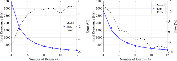
Figure 10. First natural frequencies of two sets of OS structures with 4–12 beams showing error between model prediction and measurement for (a) outer beam fixed, and (b) center beam fixed.
Download figure:
Standard image High-resolution imageUnlike the PZ and OS prototype designs, the SZ prototype was made with the ability to disassemble and reassemble. The beam segments were aluminum having a width of 25.4 mm, a free length (distance between joint blocks) of 12.32 cm, and a thickness of 3.02 mm. The joint blocks were steel cubes having a depth (b) dimension in figure 6(b) of 25.4 mm, a centroid distance  of 12.7 mm, and a mass of 55.2 g. A photo of the SZ prototype used for experimental validation is shown in figure 8(c). Natural frequencies of the SZ were measured for a single beam up to 5 beam segments both with and without an additional tip mass. A joint block (55.2 g) was used as the tip mass. Comparisons between these measurements and model predictions are summarized in figure 11 which shows excellent agreement between model and experiment especially for the case with a tip mass where the error never exceeds 1%.
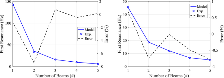
Figure 11. First natural frequencies of two sets of SZ structures with 1–5 beams showing error between model prediction and measurement for (a) no tip mass, and (b) tip mass.
Download figure:
Standard image High-resolution imageThe majority of all error in the previously discussed model comparison results can be attributed to beam segment length measurement error, imperfect clamping conditions, and oversimplified joint conditions between each beam segment. For example, the joint blocks of the SZ structure are assumed to be rigid, when in reality, they are elastic. Also, it is assumed that each planar structure (PZ an OS) can be represented as a series of lines drawn down the center of each beam segment. Given this centerline representation of the PZ and OS structures, the exact stiffness and mass distribution of the joints between beam segments are not accounted for, thus causing some error. Additional error can be attributed to unaccounted for Poisson's effect and shear deformation in beam segments with small aspect ratios.
4. Performance comparisons
This section uses the proposed models to investigate how the four periodic structures discussed in this paper compare in terms of strain distribution, and geometric compactness. Results of a brief computational efficiency analysis are also discussed. Here, the proposed model is compared to commercially available finite element analysis software.
4.1. Strain distribution and design compactness
The following analysis considers four structures of similar overall size, material properties, and beam segment dimensions. The structure types are those of the previously discussed PZ, OS, and SZ. For convenience, OS structures will be classified as two types: outer beam fixed (OSo) and inner beam fixed (OSi) as illustrated in figure 4. All structures are made with aluminum 6061-T6 and have a beam segment width and thickness of 5.08 mm and 1.52 mm respectively. The distance between adjacent PZ and OS beam segments is 1.02 mm. There are no tip masses and the SZ joint block masses are 2.55 g.
One performance metric considered for both metastructure and energy harvesting applications examines how strain is distributed throughout the entire structure. It is a more efficient use of volume and mass to have strain evenly distributed through the entire structure rather than locally concentrated. Given the mode shape  the single-sided absolute surface strain of each beam segment can be defined as,

where 
 and
and  are the thickness, length coordinate, and length of the
  beam segment respectively. Upon normalizing
  by the maximum absolute strain and dividing by the number of beam segments, the average strain distribution can be defined as,

which is equal to one if the absolute surface strain in all segments is equal. This strain distribution metric is low if the highest strains are experienced in a smaller percentage of the structure. For comparison, the first mode of a uniform cantilever beam has a strain distribution value of 0.393.
Figure 12 shows a series of strain distribution values calculated using equation (61) while increasing the number of beam segments over a range from 3 to 30. The best (largest value) strain distribution was initially achieved with the OSi; however, the PZ performs better for  Compared to all other designs, the OSi has the best strain distribution for
  which appears to stabilize at 0.54 while that of the PZ, OSo, and SZ structures decays steadily as
  increases. Strain distribution for the OSo and SZ structures is already less than that of a EB beam at only 5 and 3 beam segments respectively.
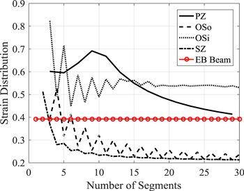
Figure 12. Strain distribution for each type of periodic structure as a function of number of beam segments compared to that of a Euler–Bernoulli beam.
Download figure:
Standard image High-resolution imageThis vast difference between the two OS-type structures can be explained by considering which beam segments must support the most weight under a static loading condition. The OSi has the best overall strain distribution because the shorter stiffer beams (nearest the fixed beam) support the entire structure. Unfortunately for the OSo, a majority of the strain is in the longest softest beam segment while segments closer to the center of the structure experience negligible strains.
Although the SZ and OSo structures have poor strain distributions, they should not be ignored nor considered poor designs overall. There may be instances where strain distribution is not the most important design factor. For example, the SZ structures considered in this section have a natural frequency approximately an order of magnitude lower than the OSo and OSi structures and nearly half that of the PZ structure. While it has such low natural frequencies, the SZ structure has the largest overall volume which is nearly an order of magnitude greater than that of the OSo and OSi depending on the number of beam segments.
Given these various advantages and disadvantages of each structure type, another design metric is proposed in an attempt to provide a fair performance comparison. This design metric is a measure of total surface strain normalized by the maximum strain, natural frequency, and volume. This total strain density metric can be expressed as,

where  is the overall volume required to encase the structure,
  is the natural frequency,
  is the maximum surface strain in the structure, and
  is the single-sided absolute surface strain defined in equation (60). The strain density metric can be related to the energy density in energy harvesting terms. Also, both energy harvester and metastructure designs seek to minimize resonator volume and natural frequency which are well-known competing design goals. Therefore, this strain density metric increases with increasing total normalized strain, decreasing natural frequency, and decreasing volume.
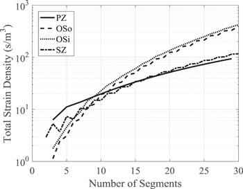
Figure 13 summarizes the total strain density calculations made with equation (62) for the PZ, OS, and SZ structure types. Comparing these strain density results reveals that the PZ structure is the best choice for  where it is then surpassed by the OSi structure for
  then the OSo for
  then lastly by the SZ for
Figure 13. Comparison of total strain density metric for each type of periodic structure as a function of number of beam segments.
Download figure:
Standard image High-resolution image
4.2. Computational efficiency
In order to demonstrate the efficiency of the proposed models, a simple comparison was performed on a 12-beam OS beam using ANSYS finite element analysis software and MATLAB. Calculations were performed on a computer having 16 GB of RAM and a quad core processor running at 3.6 GHz. ANSYS was setup to solve for the natural frequency and mode shape of the first mode first for a fine mesh having 4608 elements then a coarse mesh having 735 elements. Results show that ANSYS required 4.2 and 0.5 s for the fine and coarse mesh solutions respectively (not including time required to generate the mesh). Reducing from fine to coarse meshes caused the frequency estimate to increase by 0.65%. The proposed model was implemented in MATLAB where the beam segments were discretized to have the same number of elements as the two previous ANSYS models. Results of these calculations show that the complete solution (including discretization) only took 6.6 ms and 5.3 ms respectively, and caused the frequency estimate to increase by only 0.29%. In other words, the proposed model could produce 94 complete design iterations during the time it took the FEA model to produce one solution.
5. Conclusions
This research proposes a recursive modeling technique used for estimating the first natural frequency and mode shape of four types of periodic structures—PZ, OS (outer beam fixed), OS (inner beam fixed), and SZ. The primary goal this research is to provide a more efficient means of estimating first mode dynamics of periodic structures in an attempt to minimize modeling complexity and computational effort for future design optimization. The types of structures represented by these models were chosen based on their growing popularity in the energy harvesting and metastructures literature. Therefore, a secondary goal of this research is to use the proposed models to provide insights on the primary advantages and disadvantages of various periodic structure designs.
Each proposed model was first validated with experimental measurements performed on numerous prototypes of each structure while varying the number of beam segments. Results of this validation study demonstrated excellent agreement between model prediction and measurement. For most cases, the error between model and experiment did not exceed 2%. The primary sources of error were identified as beam segment length measurement error, imperfect clamping conditions, and oversimplified joint conditions between each beam segment. Additional sources of error were attributed to unaccounted for Poisson's effect and shear deformation in beam segments with small aspect ratios.
Lastly, the proposed models were used to assess the performance of each of the four structure types with regard to volume, natural frequency, and strain distribution. Overall, OSi structures were shown to perform the best by having the most uniform strain distribution and lowest volume. In a few cases however, it was shown that the PZ structure outperformed the OSi. Other notable advantages and disadvantages of the four periodic structure types discussed are as follows. First, SZ structures were shown to have natural frequencies approximately an order of magnitude lower than the OSo and OSi structures and nearly half that of the PZ structure. Next, while it had such low natural frequencies, the SZ structure also had the largest overall volume which was nearly an order of magnitude greater than that of the OSo and OSi depending on the number of beam segments.
Immediate related future research will focus on performing an in-depth optimization study across a vast design space using the recursive models proposed in this work. This future optimization analysis will consider maximum stress limitations, strain distribution, tip mass effects, number of beam segments, overall dimensions, and dimensions of each beam segment.
Acknowledgments
The authors would like to extend their sincere gratitude for the funding of this research provided by both the University of Michigan, College of Engineering, and the US Air Force Office of Scientific Research under the grant number FA9550-14-1-0246 'Electronic Damping in Multifunctional Material Systems' monitored by Dr BL Lee.