

Abstract
Recent studies have shown that tuning a dielectric barrier discharge (DBD) in the medium-frequency range (MF: from 0.3 to 3 MHz) allows a low-power and a high-power mode to be sustained. In the present article the effect of the driving frequency on a DBD is studied from the low-frequency range (LF: from 30 to 300 kHz) to the high-frequency range (HF: from 3 to 30 MHz). This is achieved using fast imaging together with electrical and spectroscopic diagnostics. At every frequency, a diffuse discharge is sustained. It is observed that at 25 kHz the discharge is an atmospheric-pressure glow discharge (APGD) while at 15 MHz the discharge behaves as a capacitive discharge in the RF-α mode. The usual LF APGD behavior is observed up to 100 kHz. Above 200 kHz, the positive column remains during the whole cycle so that the hybrid mode is sustained. At 5 MHz, the hybrid mode finally turns into the RF-α mode. In addition to the LF APGD, RF-α and hybrid modes obtained when the applied voltage is significantly higher than the ignition value, two other modes can be reached at low applied voltage. A Townsend-like mode is achieved from 50 to 100 kHz while in the medium-frequency range, the Ω mode is sustained. Moreover, only from 1.0 to 2.7 MHz there is a large hysteresis occurring when the discharge transits back and forth from the Ω to the hybrid mode. It is also found that when the frequency increases from 25 kHz to 15 MHz, the rms current increases over two orders of magnitudes while the rms voltage decreases by about 60%. The gas temperature estimated from N2 rotational spectra is always close to room temperature but the discharge is more energy efficient (in the HF range) as a lower fraction of energy turns into gas heating.
Export citation and abstract BibTeX RIS
1. Introduction
Since the mid 1980s, dielectric barrier discharges (DBDs) have been known to be an efficient way to generate diffuse discharges at atmospheric pressure [1–3]. Since then, studies have mainly focused on two intervals of the radio-frequency range, namely, the low-frequency range (LF), defined as 30–300 kHz (in practice, often including frequencies below) and the high-frequency range (HF) defined as 3–30 MHz. In the low-frequency range, helium DBD typically give rise to an atmospheric pressure glow discharge (APGD) that is similar to the low-pressure DC discharge [4]. It features a positive column and a cathode fall that oscillate according to the excitation frequency. The light intensity is usually maximum close to the cathode. Low frequencies also give rise to the atmospheric-pressure Townsend discharge (APTD) [5]. Typically, in nitrogen gas, the APTD is characterized by its low ion density. Consequently, the applied electric field is undisturbed by the low space charge in the gas and the light intensity is maximum close to the anode.
On the other hand, in the high-frequency range, the discharge is usually identified as a radio-frequency (RF) discharge. Diffuse atmospheric-pressure discharges are mainly categorized in three different modes: the α mode [6, 7], the Ω mode [8] and the γ mode [9, 10]. The first two ones rely on Ohmic heating. In this case, the electron density is always maximum in the middle of the gas gap (if recombination is neglected). Then the light emission is maximum in the sheaths (close to the solid surfaces) or in the middle of the gas gap whether the space charge modifies the electric field significantly or not. This gives rise to the α or the Ω mode respectively [11]. The third diffuse discharge mode that is sustained in the HF range is characterized by a large contribution of secondary electrons emitted at the solid surface. The ion density is then maximum in the sheaths while the light emission is concentrated very close to the solid surface.
While the discharge behavior is well understood for frequencies in the LF and the HF range, only a very few studies were performed for the frequency band in-between, namely the medium-frequency range. According to the International Telecommunication Union the medium frequency (MF) range spreads from 0.3 to 3 MHz [12, 13]. In plasma physics, this frequency band is a transitory region between low and high frequencies. In an atomic gas, below the MF range, the electric field oscillations are slow enough for the charged species (electrons and He or He2 ions, in the case of an helium discharge) to follow it. On the other hand, above the MF range, ions might be considered static while the electrons oscillations are dramatically reduced. Accordingly, plasma scientists often refer to LF range when ions can follow the electric field (typically below 300 kHz, including the very low-frequency (VLF) range, etc) and HF range when ions are approximately static (typically above 3 MHz). Therefore, the aim of the present study is to investigate the behavior of a DBD over a frequency range spanning from LF to HF.
Previous studies on the effect of the frequency on a helium diffuse DBD were focused on the low or the high-frequency range separately [14–19]. In argon and ammonia Penning mixture, some studies were carried over a wide frequency range [20–22]. However, the gas nature and the DBD configuration often give rise to different behaviors. In a previous paper, we showed that in a helium DBD, two diffuse discharge modes can be sustained in the MF range, namely the Ω mode and a mode showing an emission pattern similar to that of the RF-α mode [23]. These two modes are obtained in the same experimental conditions except for the applied voltage. While our previous endeavors were focused on identifying these discharge modes between 1.0 and 2.7 MHz, in this paper, we investigate the discharge behavior beyond the boundaries of the medium-frequency range. The frequency is therefore varied from 25 kHz to 15 MHz while the rms applied voltage is varied from 190 to 850 V. Section 2 describes the experimental setup while sections 3 and 4 are devoted to results and analysis of time-averaged and time-resolved discharge diagnostics respectively. Finally, results are interpreted and discussed in section 5.
2. Experimental setup
The plasma reactor consists of a plane parallel DBD with one solid dielectric on each electrode. The discharge cell is placed in a chamber connected to a mechanical pump aiming to minimize the amount of impurities. Experiments are thus performed in a well-controlled atmospheric environment at a pressure of 101.3 kPa with a constant helium flow (99.999% purity) of 8.3 × 10⁶ m3 s−1 through a 2 mm gap between the alumina solid dielectric surfaces. The linear flow speed is about 0.06 m s−1, a value that is sufficient to ensure a gas refresh rate that allows the impurities to be limited. More precisely, in another paper, the impurity percentage was estimated using the time constant of the helium metastable atoms density determined during the afterglow of the discharge at 50 kHz (in the same conditions as here), i.e. 2.3 μs. The quenching of the metastable atoms corresponds to that caused by either 15 ppm of water impurities or 130 ppm of air impurities [24].
The electrodes cover a symmetric area of 10 mm × 50 mm on each dielectric (solid dielectric thickness of 1 mm). With respect to figure 1, the gas is flowing along the x axis across the 10 mm electrode length. In order to achieve frequencies ranging from 25 kHz to 15 MHz, three distinct power supply systems are employed. In each case, the waveform generator (Agilent 33220A) delivers the corresponding sinusoidal voltage to a power amplifier. However, the power amplifier and the matching circuit depends on the targeted frequency. Table 1 enumerates the frequencies tested along with the corresponding power system.
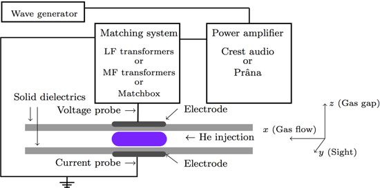
Figure 1. Discharge cell and electrical circuit. The gas is flowing along the x axis, from the right to the left. The gas gap of 2 mm between the dielectrics lies along the z axis, while the line of sight of the optical measurements (camera and spectrometers) lies along the y axis.
Download figure:
Standard image High-resolution imageTable 1. Frequencies tested and the power supply systems used to tune it. Frequencies ranging from 25 to 125 kHz are amplified by a Crest Audio amplifier (CC4000) matched with a transformer. Frequencies ranging from 150 to 5000 kHz are amplified by the Prâna amplifier (GN 500) and matched using a set of noncommercial transformers. The frequency is tuned to be at the resonance of the system made by the transformer and the discharge cell [22]. Frequency variation induces voltage amplitude variation, however, for a given frequency, the voltage amplitude can be varied by changing the waveform generator voltage amplitude. In this case, the exact frequency is very sensitive to the quality of the connexions (noncommercial soldering). Consequently, the frequency can vary up to 3% of the indicated values. From 10 MHz and beyond, the same Prâna amplifier is used but the transformer is replaced by an Advanced Energy (Navio) digital matching network allowing to tune the frequency.
| Frequencies (kHz ) | Amplifier | Matching |
|---|---|---|
| 25–50–75–100–125 | Crest Audio | Transformer |
| 150–200–280–370 | Prâna | Transformer |
| 550–730–1000–1500 | ||
| 1600–2100–2700 | ||
| 3700–4900–5000 | ||
| 10 000–11 000–12 000 | Prâna | Matchbox |
| 13 560–15 000 | ||
Current measurements are always performed with a Rogowski coil (Lilco 13W5000) located on the grounded electrode while voltage measurements are achieved with a probe (Tektronix P6015) placed on the high-voltage electrode. The latter is connected directly to the transformers secondary coil (below 10 MHz) or to the electrode cable inside the chamber (10 MHz and above, when no transformer is used). The electrical measurements are recorded via an oscilloscope of 1 GHz bandwidth (Tektronix DPO 4104). Using the electrical measurement, the power density is obtained by dividing the measured power (P)

by the measured volume ( ) of the discharge. In equation (1), f is the frequency, V(t) is the instantaneous measured voltage and I(t) is the instantaneous measured current. The volume is obtained by direct measurement of discharge lengths. While the discharge always fills the entire gap from a dielectric to the other (z axis), the discharge extent in the x and y axes are measured with rulers located in the reactor [23] (see figure 1).
In addition to the electrical measurements, the optical emission of the discharge was recorded. Time-resolved optical emission was recorded using a Princeton PI-max 2 camera (300–900 nm). An optical filter (center wavelength at 707 nm and bandpass of 10 nm FWHM) was occasionally added in front of the camera in order to measure the emission of helium at 706.4 nm: He(33S → 23P). The emission spectra were recorded by a Maya 2000-Pro spectrometer system (165–1100 nm) including a Hamamatsu S10420 Detector. A Princeton instrument Acton SP2500 spectrometer equipped with the PI-max 2 camera was also used to record rotational spectra of N2( ) in order to estimate the gas temperature. In each case, the light was collected along the y axis, perpendicularly to the gas flow direction.
3. Time-averaged characterization
In this section, we provide an overview of the discharge behavior in the complete range of experimental parameters, i.e. from 25 kHz to 15 MHz and from 0 to 850 Vrms. Differences as well as similarities are highlighted via electrical and emission spectroscopy characterizations. Then, temperature measurements are discussed with respect to selected frequencies.
3.1. Identification of discharge modes
To illustrate the extent of the diffuse conditions, figure 2 shows the rms current and voltage evolution for most of the frequencies available. The  curves are obtained by increasing the voltage of the waveform generator while measuring the rms voltage and current. Experiments always started at 0 V of applied voltage and stopped before leak discharge or instabilities could occur (arbitrary upper boundary). Let us note that the illustrated data were recorded only during the increase of the applied voltage. Additional conditions are also accessible considering the decreasing part of the applied voltage. For instance, at some frequencies, it is still possible to sustain a discharge significantly below the breakdown voltage (see section 5). Based on long exposure camera measurements together with oscillograms of current and voltage, the discharge is always found diffuse except between 3.7 and 4.9 MHz where the discharge displays some instabilities when high voltage is applied. Diffuse conditions are represented by open symbols in figure 2.
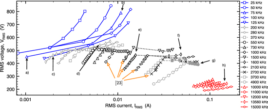
Figure 2.
 characteristic curves for different frequencies from 25 kHz to 15 MHz. Blue solid lines indicate frequencies for which the behavior is typical of the LF range (including 25 kHz in the VLF range), black dotted lines indicate frequencies for which the discharge behavior is typical of the MF range and red dashed lines indicate frequencies for which the discharge behavior is typical of the HF range. Gray lines indicate transitory frequencies for which the discharge behavior is unclear. The letters indicate the current and voltage associated with pictures in figure 3. The curves indicated by orange arrows are those already reported [23].
Download figure:
Standard image High-resolution imageAlthough precise quantitative analysis of the  curves would require to consider the discharge current and the voltage applied to the gas instead of the measured current and voltage, important information with respect to the classification of the discharge modes can be found in figure 2. For instance, inflections of the
  curves of figure 2 can be interpreted as major change in the discharge behavior, i.e. mode transitions. Accordingly, figure 3 shows examples of gas gap pictures (wavelength integrated from 300 to 900 nm) for different
  conditions reported in figure 2. Power density is indicated on the pictures to better compare conditions at different frequencies. From these images only two emission patterns can be distinguished: either emission is concentrated in the bulk or it is concentrated in the sheath regions. Actually, emission is concentrated in the bulk from 50 kHz to 4.9 MHz, when the applied voltage is close to breakdown voltage (up to inflection). For every other conditions the light emission is concentrated close to the solid dielectrics. This is after inflection (when it exists) or during the whole curve (when no inflection occurs). Let us note, that picture 3(g) exhibits instabilities that occur at 3.7 and 4.9 MHz when the applied voltage is high enough.
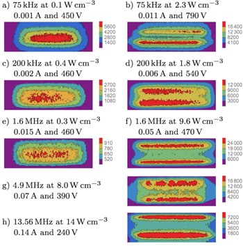
Figure 3. Pictures of the discharge for different frequencies and power densities corresponding to the labeled  data of figure 2. Exposure varies from 1 to 100 ms. Intensities in arbitrary units are indicated at the right of each picture.
Download figure:
Standard image High-resolution imageGoing back to figure 2, one can foresee some discharge modes with respect to the inflections of the  curves. Whatever the frequency is, we will refer to the low-power mode before the
  inflection i.e. when emission takes place in the gas bulk. Similarly, we will refer to the high-power mode after the
  inflection, when the light is emitted close to the dielectric surfaces. In the low-frequency range (solid blue lines), the inflection of the
  curve gives rise to the low-power LF and to the high-power LF modes. In the MF range (dotted black lines), the inflection of the
  curve gives rise to the low-power MF and the high-power MF modes. Finally, from 10 MHz and above (dashed red lines), when no inflection occurs in the
  curves, the corresponding mode will be referred as the high-power HF mode. The boundaries of these modes with respect to the frequency are difficult to identify in figure 2. Consequently, the gray lines represent transitions for which the classification of the modes are still to be determined. Discharge modes are roughly indicated in table 2.
Table 2.
Discharge classification based on  inflections and long exposure pictures.
| LF range | MF range | HF range |
|---|---|---|
| 25–100 kHz | 0.2–3 MHz | 5–15 MHz |
| Low-power LF | Low-power MF | |
| High-power LF | High-power MF | High-power HF |
Before deploying efforts to understand the mechanisms underlying these discharge modes and investigating their boundaries, we briefly comment some spectroscopic features of the discharge modes.
3.2. Spectrally-resolved discharge emissions
Even if the discharge behavior is completely different when the frequency grows from 25 kHz to 15 MHz, some features are quite similar, as illustrated by the time integrated spectra shown in figure 4. The same emitting species are present in all spectra. Significant intensity of OH( ) (λ = 306.4 nm), N2(C
 ) (λ = 337.8 nm) and
  (B
(B
 ) (λ = 391.4 nm) molecular bands as well as He(33S → 23P) (λ = 706.4 nm) and O(
 ) (λ = 777.5 nm) atomic lines are observed. We note that while the lines present in the visible spectrum are the same for each frequency and power density, their ratios can vary substantially with respect to experimental parameters (e.g. figure 4(a) compared to (b)). While the plasma composition should be constant whatever the frequency is, this suggests changes in the electron dynamics.

Figure 4. Optical emission spectra corrected by the response curve of both spectrometer and detection system for the discharge at (a) 50 kHz for 1.7 W cm−3 and (b) 10 MHz for 9.6 W cm−3.
Download figure:
Standard image High-resolution imageThe emission at 706.4 nm is the strongest one among helium emissions and it can easily be detected in all conditions. Therefore, in the following sections, many experimental investigations will be devoted to this transition. In order to understand the upcoming results, let us note that the He(33S) state can be populated by three main mechanisms, namely direct electron impact on helium ground state (threshold energy of 22.7 eV) [25], electron impact with He(23S) metastable state (threshold energy of 2.9 eV) [26] and dissociative He2+ recombination with low-energy electrons [27]. Therefore, the presence of the He(33S → 23P) emission should be related to either a significant concentration of electrons with energy higher than 22.7 eV or a few high-energy electrons compensated by a significant concentration of metastable atoms or He2+ ions. For a deeper discussion on the observed transitions and the origin of their emission, see [23].
The emission from nitrogen molecule, N2(C
 ), is also present in all of the conditions tested. Its presence is usually associated with impurity desorption from the solid dielectrics [28]. In fact, N2(C
 ) has been used as a thermal probe in similar cases [23, 29, 30]. Here, the transition N2(C
 ) is used as a thermal probe via rotational spectroscopy. By fitting the recorded rotational spectra with the Specair program [31], we calculated the gas temperature by multiplying the fitted rotational temperature by 1.095 (rotational factor correction of the ground state [32]). By means of a thermocouple probing the dielectric surface near the electrode area, the dielectric temperature (Tdie) was also recorded. Both measured temperatures are shown for selected frequencies in figure 5.

Figure 5. Dielectric temperature (Tdie) and gas temperature from N2(C
 ) rotational spectra (Tgas) as a function of the power at different frequencies. The rotational spectra are spatially integrated and the exposure varies between 100 and 1000 ms. The rotational temperature is obtained by fitting the experimental spectra to simulated spectra generated by the Specair program. Dielectric temperatures are measured with a thermocouple placed near the discharge zone between the solid dielectrics. The inset is a magnification of the zone of low power and low temperature. Uncertainties are about 3 and 50 K for dielectric and gas temperature respectively.
Download figure:
Standard image High-resolution imageFigure 5 shows that, at each frequency, both rotational and dielectric temperatures increase with power. Whatever the frequency is, at the lowest power, the dielectric temperature is at room temperature and the gas temperature calculated from N2 rotational spectra is slightly lower (likely due to the gas temperature drop from the pressure release between the gas bottle and the reactor). In the LF range, at 100 kHz, the gas temperature increases very steeply up to 360 K with the power while the dielectric temperature is constant at 300 K. This suggests that, in the LF range, surface cooling by the helium feed at room temperature is more efficient than surface heating by the discharge. For frequencies in the MF range (e.g. at 1 and 1.6 MHz), both temperatures vary in a similar manner. Their variations are clearly related to the discharge modes: low-power and high-power MF modes. In this case, the gas temperature maximum is 400 K and the maximum dielectric temperature is 335 K. Finally, in the HF range, for 13.56 MHz, both temperatures are almost constant. In agreement with discharge in similar conditions (HF range in pure helium), the gas temperature does not exceed 300 K [33].
4. Time-resolved characterization
In this section, time-resolved light emission is investigated as a function of the frequency. In order to facilitate the discussion, we will first consider the case of the high-power modes, and then the low-power modes.
4.1. High-power discharge modes
In order to describe the basic mechanisms behind frequency transitions, let us consider the time-resolved optical emission (wavelength integrated from 300 to 900 nm). Figure 6 shows the spatio-temporal distribution of the spectrally integrated emission along the gas gap over one cycle for various frequencies from the LF to the HF range. The high-voltage electrode lies above the solid dielectric located at 2 mm (along the z axis) while the grounded electrode lies below the solid dielectric located at 0.0 mm. To represent the light distribution from one electrode to the other as a function of time, each picture is integrated along the direction parallel to the gas flow (the x axis) and the results are adjoined to get the variation of the spatial distribution of the light from an electrode to the other as a function of time. Results are presented over one cycle. Each figure is made from at least eight pictures and time resolution is increased from 100 to 15 ns when the frequency increases. The first picture of a series is triggered when the measured voltage intersects 0 V towards positive values. This means that the upper electrode is the anode for the first half-period and the cathode for the second half-period.

Figure 6. Time evolution of the light emission along the gas gap over one cycle for high-power modes at different frequencies. The first picture acquisition is synchronized with the measured voltage intersection with zero, making the upper electrode positive during the first half-period. Each measurement is recorded with a different number of accumulations and exposure time varying from 200 to 20 000 and from 15 to 100 ns respectively. Every recording is on the same scale as intensities are corrected by the number of accumulations and the exposure. A schematic of the images indicates relevant gap zones and the position of the transient anode and cathode.
Download figure:
Standard image High-resolution imageConsidering the optical emission spectrum of the discharge in figure 4 and the spectral response of both camera and lens (more sensitive in UV than in visible), the light emission of figure 6 should represent mainly OH(A ), N2(C
 ), and
  (B
(B ). While OH(A
 ) and
) and  (B
(B ) are mostly populated by stepwise excitation using helium metastable atoms, N2(C
 ) is usually populated by direct excitation [23, 25]. Accordingly, the emission recorded in figure 6 represents the excitation from various contributions (direct excitation, stepwise excitation, etc) and can barely be associated with the ionization rate. Nonetheless, let us describe figure 6 with respect to the discharge modes previously suggested from LF to HF:
- (i)High-power LF mode. First, at 25 kHz (figure 6(a)), the discharge exhibits features expected from a typical LF APGD [4, 34]: the maximum light emission occurs on the cathode side and, during the discharge development, light emission propagates mostly from the anode to the cathode. At each position in the gas gap, the emission falls below 10% of the maximum value over about 20% of the cycle suggesting that very few energetic species remain in the gas between two pulses. From 50 kHz, the discharge behavior starts to slightly deviate from that of a typical LF APGD. While the maximum intensity value is similar to that of 25 kHz, the emission intensity never falls below 10% (on the whole gap) because of the reduction of the half period. We observe that the tail of the glow at the cathode connects to the ignition of the following pulse in the spatial region newly became the anode side. There is still a region where the emission is below 10%, namely the anode side before it becomes the cathode side. At 100 kHz (figure 6(c)), not only the tail of the cathode region connects to the anode region half a cycle later but it also connects to the cathode region one complete cycle later. Only in the bulk there is a small delay during which the emission is below 10% of the maximum. However, the discharge is still clearly a LF APGD as the pulse grows from the anode to the cathode and the maximum emission is on the cathode side.
- (ii)Transition. At 125 kHz (figure 6(d)), the emission pattern becomes more spatially symmetric, i.e. the emission does not grow simply towards the cathode. The emission starts from the sheath region and increases from the middle of the sheaths towards both the dielectric surface (cathode side) and the bulk. On the other hand, the intensity of the sheath falls as low as 20% of the maximum, illustrating the still largely fluctuating emission.
- (iii)High-power MF mode. At 200 kHz (figure 6(e)), the cycle duration is 500 ns. The intensity fluctuation during the cycle becomes very weak (about 50% of the maximum intensity in the sheath). In addition, the light emission of the bulk is almost constant over the whole cycle. This suggests that the positive column of the APGD is now very homogeneous over the time-period. Let us note that the maximum emission is always on the cathode side while no relative maximum appears on the anode side, hence, the emission on the anode side should only be due to the long-lived species that remains from the previous cycle. Because of its continuous positive column and light evolution from the sheath region towards both the bulk and the dielectric surface, this mode can no longer be identified as an APGD (in the LF APGD sense [35]). However, since there is no relative maximum on the anode side (α mode signature), it cannot be identified as the RF-α mode either. Therefore, we will refer to this mode as the hybrid mode. A similar behavior occurs up to 1.6 MHz. However, at 1.6 MHz, the power density is significantly higher than at lower frequencies in the MF range. The light emission is also slightly closer to the solid dielectrics. This corresponds to one of the
 curves with an rms current jump in figure 2. In fact, even if the light emission proposes that the same discharge mechanism underlies the discharge from 200 kHz to 2.7 MHz, the discharge mode appears to be slightly different below and above 1 MHz.
 - (iv)Transition. Between 2.7 and 5 MHz, according to figure 3(g) there is a transition region. However, no time-resolved data was recorded in this range.
- (v)High-power HF mode. From 5.0 MHz (figure 6(j)), the α mode is finally well established. The emission becomes more symmetric between the anode and the cathode, i.e. there is a relative maximum on both sides at about the same time. This is similar to the RF-α mode of atmospheric-pressure discharges in helium [33, 36]. In addition, this mode is identified as α rather than γ on the basis of the following arguments: (1) the observed ratio between the intensity near the surfaces and the intensity in the bulk is much lower than in the γ mode [36, 37], (2) the recorded light emission is located much farther from the surface than it would be in the γ mode [36, 37], and (3) the measured light emission pattern displays the same space and time relative maxima than the simulated electric field [8]. Let us note that, the same behavior is observed at 13.56 MHz (figure 6(k)) although the time resolution of the recorded data is not as good as for other frequencies because of the shorter time-period (73.7 ns).

A better understanding of the discharge evolution can be reached from the helium He(33S → 23P) emission as a function of the frequency. This emission is measured with a 10 nm bandpass filter centered on 707 nm. Using the same procedure as for figure 6, figure 7 shows the spatial distribution of the helium emission along the gas gap.
- (i)APGD mode. At 25 kHz, the helium emission grows from the anode to the cathode and no emission is detected during a significant part of the time-period. This is quite similar to the integrated emission shown in figure 6(a) with the difference that the helium emission last for a shorter period of time than the integrated emission.
- (ii)Hybrid mode. At 550 kHz, unlike the integrated emission, the helium emission is neither connected in space nor in time and falls below the detection level between two half-cycles. We note that the emission starts from the sheath regions and grows towards both the bulk and the dielectric surface but in contrast to the integrated emission, no significant helium emission is recorded on the anode side. Above 500 kHz (1/f ≤ 2 μs), assuming that the density of helium metastable atoms is almost constant during the whole cycle and across the entire gas gap (the lifetime of He(23S) metastable atoms was measured to be 2.3 μs by using a diode laser [24]), the He(33S) state should be easily populated by stepwise excitation. As a consequence, the absence of He(33S → 23P) emission on the anode side suggests that unlike the RF-α mode [8], ionization does not occur significantly in this region (see figure 7(c) for comparison).
- (iii)RF-α mode. At 5.0 MHz, the helium emission is maximum on the cathode side (similarly to all other frequencies in their high-power mode). However, in agreement with ionization rate simulated in similar conditions [8], there is a small increase of the helium emission on the anode side. This suggests that the hybrid mode is different than the RF-α mode. Let us note that the signal to noise ratio is not as good as for other frequencies.
Finally, in order to compare the hybrid mode to the APGD mode, the decay of the He(33S → 23P) emission as a function of time is illustrated in figure 8 for both the APGD and the hybrid modes. Emission at the position z = 1.5 mm (see figure 7) is considered with t = 0 μs chosen at the maximum intensity. Since the He(33S) state is radiative, it is expected that its loss is controlled by spontaneous emission (collisional quenching can become important at atmospheric pressure but it should be the same in every condition under investigation). Then, the intensity should be proportional to the population of He(33S) which should depend on the electron density and metastable density as the He(33S) is created by electron collisions from the fundamental level or from the metastable level by a two-step process. In figure 8, very different behaviors are observed for frequencies above (figure 8(b)) and below or equal to 100 kHz (figure 8(a)). From 200 kHz, the usual exponential decrease is replaced by a slower decrease. This occurs when the time scale of the memory effect shifts from half a cycle to a full cycle, resulting in a longer accumulation of different species which induce higher densities. Thus, a possible explanation for this observation is that the recombination of He2+ and electrons significantly participate to the population of He(33S) when the memory time scale increases. However, when the frequency increases from 200 to 1000 kHz, the He(33S → 23P) decays faster while still governed by the same decreasing function. This could be explained by the lower electron energy considering that the ignition phase is reduced, thereby reducing the contribution of direct and stepwise excitations in the He(33S) population.
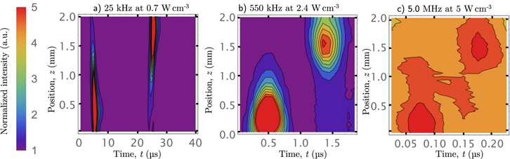
Figure 7. Time evolution of the helium He(33S → 23P) emission along the gas gap. The acquisition of the first picture is synchronized with the measured voltage intersection with zero, making the upper electrode positive during the first half-period. Each measurement is recorded with a different number of accumulation and exposure: (a) 25 kHz for 100 ns gate width and 40 000 accumulations, (b) 550 kHz for 50 ns gate width and 20 000 accumulations and (c) 5.0 MHz for 25 ns gate width and 10 000 accumulations. Every recording is on the same scale as intensities are corrected by the number of accumulation and the exposure.
Download figure:
Standard image High-resolution image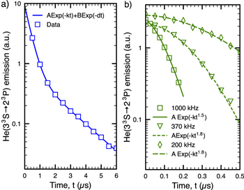
Figure 8. Decrease of the He(33S → 23P) emission intensity at z = 1.5 mm as a function of time. Data extracted from figures similar to those of figure 7. (a) APGD mode at 25 kHz and 0.7 W cm−3. (b) Hybrid mode at 1 MHz, 370 and 200 kHz.
Download figure:
Standard image High-resolution image4.2. Low-power discharge modes
When the applied voltage is close to its breakdown value and the frequency lies between 50 kHz and 2.7 MHz, the spectrally-integrated emission is concentrated in the bulk (see figure 3). In order to investigate the behavior of the discharge in such conditions, let us consider time-resolved optical imaging. Figure 9 shows the spatial distribution of the spectrally integrated emission along the gas gap.
- (i)Low-power LF mode. At 100 kHz, one observes that the emission is stronger on the anode side than on the cathode side. This behavior significantly differs from the APGD at 100 kHz depicted in figure 6(c). To be more precise, let us consider the He(33S → 23P) transition. This is achieved in figure 10 where the time evolution of the distribution of He(33S → 23P) line emission along the gas gap is illustrated at 100 kHz. Helium emission reaches a maximum at the anode with a strong increase from the cathode. This behavior is similar to the APTD and can be explained by a quasi-uniform electrical field in the gap. As the electron energy is constant over the gap, emission is maximum where the density of electrons is the highest, i.e. at the anode [38]. This suggests that the ion density is too weak to enhance the electric field locally and form a cathode fall. Such a behavior is a characteristic of APTD and the corresponding mode will be refered as APTD-like (APTD-L) mode.
- (ii)Transition. Between 100 and 200 kHz, there is a transition region. However, no time-resolved data was recorded.
- (iii)Low-power MF mode. From 200 kHz to 2.7 MHz, light emission behaves very similarly. It is concentrated in the bulk and oscillates according to the applied voltage. The emission is continuous over the whole cycle, which means that the light intensity never falls below 70% of the maximum value (at position z = 1 mm). Like for the APTD-L mode, there is no cathode fall signature and the ion density is low. In addition, the emission builds up from the bulk to the dielectrics. This behavior is in agreement with that occurring for the Ω mode [8, 11] previously reported in the MF range [23].

Figure 9. Time evolution of the spectrally integrated light emission along the gas gap. The acquisition of the first picture is synchronized with the measured voltage intersection with zero, making the upper electrode positive during the first half-period. Each measurement is recorded with a different number of accumulation and exposure varying from 200 to 20 000 and from 25 to 100 ns respectively.
Download figure:
Standard image High-resolution image
Figure 10. Time evolution of the distribution of He(33S → 23P) line emission along the gas gap. The acquisition of the first picture is synchronized with the measured voltage intersection with zero, making the upper electrode positive during the first half-period. The frequency is 100 kHz and the power density is 0.09 W cm−3. The pictures were recorded with 200 000 accumulations and exposure of 1 μs.
Download figure:
Standard image High-resolution image5. Discussion
In section 3, we defined possible discharge modes as a function of the power they absorb and the approximate range of frequency in which they could be obtained. With the help of fast imaging, these modes were identified as APGD, APTD-L, Ω, hybrid and RF-α modes. This allows us to convert table 2 into table 3 in which the discharge modes are now pointed out. Before undertaking a more specific classification, let us consider a novel analysis of the rotational temperature and a brief comment about the discharge modes in the MF range.
Table 3. Discharge modes observed from 25 kHz to 15 MHz.
| LF range | MF range | HF range | |
|---|---|---|---|
| 25–100 kHz | 0.2–3 MHz | 5–15 MHz | |
| Low power | APTD-L | Ω | |
| High power | APGD | Hybrid | RF-α |
5.1. Effect of the frequency from LF ot HF
In section 3.2, the gas temperature in the discharge was obtained at several frequencies. Going back to the rotational temperature of N2, one observes that for each mode at each frequency, the rotational temperature increases linearly with the power. The slopes S(f) of these curves were calculated and are presented in figure 11 as a function of the frequency. The slope of the rotational temperature as a function of the power corresponds to the amount of injected energy converted into rotational energy. In other words, the higher S(f) is, the higher is the power loss to increase the rotational temperature. Therefore, figure 11 indicates that as S(f) decreases with the frequency, less energy is converted into rotational temperature at higher frequencies.
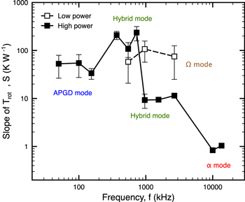
Figure 11. Trot(P) slope as a function of the frequency for different modes. The rotational temperature was recorded from N2(C
 ) spectra fitted to simulated spectra (with the help of Specair). Error bars represent the error on the fitted slope S(f).
Download figure:
Standard image High-resolution imageFigure 11 shows that S(f) varies over three orders of magnitude in the frequency range investigated. It is also clearly correlated to the discharge mode. While the value of S(f) decreases from the APGD mode, to the hybrid mode (from 1 MHz and above) to the α mode, it does not seem to follow the same trend for the Ω and the hybrid (below 1 MHz) modes. For the Ω mode, both light emission and power density are very low (see figure 3(e), for instance) and the discharge should be almost purely resistive. As a consequence, the energy transfer to rotation should be important, hence leading to high S(f) values. Below 1 MHz, S(f) is also quite high in the hybrid mode. This could be explained by spontaneous oscillations (intermittent hybrid mode) that are observed between the Ω and the hybrid modes (more details about this phenomenon are provided in [24]). Since S(f) is quite high in the Ω mode, measurements corresponding to averages over the two modes should result in intermediate values (much closer to Ω mode value since the discharge spends more time in the Ω than in the hybrid mode [24]). We further note that the small difference between the value of the actual Ω mode and the intermittent hybrid mode (below 1 MHz) is not significant according to the uncertainties. In fact, the relative uncertainty on the power is much larger for the Ω and the hybrid (below 1 MHz) modes than for the other modes. Consequently, the uncertainties are actually significantly larger than the error bars shown in this mode. Finally, we note that he APTD-L mode is absent from this figure because not enough data were available to derive the slopes.
5.2. Hysteresis in the MF range
As reported in a previous study [23], an interesting feature of the MF range (f > 1 MHz) is the occurrence of a hysteresis when the applied voltage is increased and decreased in the same experiment. It was observed that during the transition from the Ω mode to the hybrid mode, the rms current jumps significantly while the measured rms voltage slightly drops. On the other hand, during the transition from the hybrid mode to the Ω mode, both the rms current and the rms voltage decrease smoothly. In the present study, we found out that this hysteresis is restricted to the hybrid mode above 1 MHz. Examples of complete  curves are shown in figure 12 where a small hysteresis is also observed at 4.9 MHz. This occurs when instabilities are observed, i.e. when the discharge is not purely diffuse (data indicated by filled symbols in figure 2).

Figure 12.
 characteristic curves for different frequencies. Black dotted lines indicate frequencies in the MF range and red dashed lines indicate frequencies in the HF range. Increase of the applied voltage is in open symbols while decrease is in filled symbols.
Download figure:
Standard image High-resolution imageFrom figure 12, it s also possible to infer that the slope of the Ω mode decreases when the frequency increases. In addition, the discharge is sustained at rms current and voltage significantly lower than the breakdown value at and beyond 10 MHz. This behavior is only observed in the HF range and is associated with the time averaged light emission becoming concentrated in the bulk. This suggests that the α mode smoothly switches to the Ω mode when the applied voltage is decreased, as expected at such frequency [8]. However, the transition is smooth so that it cannot be observed in electrical measurements in contrast to the hybrid mode.
5.3. Boundaries of the discharge modes
Based on the fast imaging pictures presented above along with the  curves of figure 2, it is possible to extrapolate the boundaries of the discharge modes. Using the power density calculated from equation (1), these modes are illustrated in figure 13 as a function of the frequency.

Figure 13. Power density of the different observed modes as a function of the frequency. Only data acquired during the increase of the applied voltage are considered (the Ω mode is not displayed in the HF range). Considering the power density jump when the frequency lies between 1.5 and 2.7 MHz, the zone delimited by the dashed lines represents the hybrid mode below the transition voltage level (during the hysteresis).
Download figure:
Standard image High-resolution image
Even though the power density in the LF range remains always lower than in the HF range, it is still convenient to separate the discharge modes in low and high power for each frequency. For the high-power discharge, we can see that the APGD is obtained up to 100 kHz. Between 100 and 200 kHz, the APGD behavior is harder to identify and the frequency range is thus better referred as transition region, which is associated with a change in the memory time scale. Up to 100 kHz, the memory effect impacts the discharge one half-cycle later, while the effect last for (at least) one complete cycle above 200 kHz. Then, the hybrid mode is observed until another transition region occurs at 3.7 MHz where the discharge exhibits instabilities. Only a few data were acquired between 5 and 10 MHz. Nonetheless, the instability region appears very narrow (between 3.5 and 5 MHz) and occurs at high applied voltage only.
For the low-power discharge, the APTD-L mode is observed in a narrow range from 50 to 100 kHz. Beyond 200 kHz, the Ω mode is already present with only a narrow region of transition between 100 and 200 kHz. The Ω mode was observed up to 2.7 MHz. However, due to the similar nature of the Ω and the α modes, it is expected that the Ω smoothly converts to the α mode as the frequency increases. This is in agreement with the conversion of the α mode the Ω mode when the applied voltage is decreased below the ignition level at frequencies above 10 MHz.
6. Conclusion
When the frequency of a helium DBD at atmospheric pressure lies in the range from 25 kHz to 15 MHz, several diffuse discharge modes are achieved. Fast imaging allowed us to identify that the discharge is sustained in five different modes: APTD-L, Ω, APGD, hybrid and α modes. As expected, the APGD and the RF-α mode are achieved in the LF and the HF range respectively. However, we found out that the APGD switches to the hybrid mode when the frequency is increased above 200 kHz. The hybrid mode is very different from both APGD and RF-α modes and is sustained up to 2.7 MHz. Above 5 MHz, the more common RF-α mode arises.
Characterized by ohmic heating, the α mode converts to the Ω mode when the applied voltage is reduced below the ignition level. However, when the frequency is decreased below 5 MHz, the α mode is no longer sustained. On the other hand, for low applied voltage, the Ω mode is sustained down to 200 kHz. Below this frequency, fast imaging shows that light emission is no longer concentrated in the bulk but rather on the anode side. This is the APTD-L mode. The transition range spreads from 100 to 200 kHz. It is defined by the memory effect that last either half a cycle or a complete cycle. Finally, the overall effect of the frequency is to increase both rms current and power while decreasing the rms voltage. The frequency also tends to increase the efficiency of the discharge since less power is converted into rotational temperature.
Acknowledgments
The authors would like to acknowledge the French 'Agence Nationale de la Recherche' (ANR), the Natural Sciences and Engineering Research Council (NSERC) of Canada and the 'Fonds de Recherche du Québec Nature et Technologies' for their financial support. One of the authors (JSB) would like to thank the Bourses Frontenac program of the Ministère des Relations Internationales of Quebec Government for cotutelle scholarship.