
Abstract
Shock ripples are ion-inertial-scale waves propagating within the front region of magnetized quasi-perpendicular collisionless shocks. The ripples are thought to influence particle dynamics and acceleration at shocks. With the four magnetospheric multiscale (MMS) spacecraft, it is for the first time possible to fully resolve the small scale ripples in space. We use observations of one slow crossing of the Earth's non-stationary bow shock by MMS. From multi-spacecraft measurements we show that the non-stationarity is due to ripples propagating along the shock surface. We find that the ripples are near linearly polarized waves propagating in the coplanarity plane with a phase speed equal to the local Alfvén speed and have a wavelength close to 5 times the upstream ion inertial length. The dispersive properties of the ripples resemble those of Alfvén ion cyclotron waves in linear theory. Taking advantage of the slow crossing by the four MMS spacecraft, we map the shock-reflected ions as a function of ripple phase and distance from the shock. We find that ions are preferentially reflected in regions of the wave with magnetic field stronger than the average overshoot field, while in the regions of lower magnetic field, ions penetrate the shock to the downstream region.
Export citation and abstract BibTeX RIS

Original content from this work may be used under the terms of the Creative Commons Attribution 3.0 licence. Any further distribution of this work must maintain attribution to the author(s) and the title of the work, journal citation and DOI.
1. Introduction
Shock waves in collisionless plasmas are ubiquitous in the Universe. Stellar termination shocks, planetary and stellar bow shocks, and intergalactic shocks all act to slow down and thermalize supersonic plasma (Tsurutani and Stone 1985). Collisionless shock waves are also powerful particle accelerators. Shock waves caused by the fast ejecta from supernova remnants are the most likely source of the high energy cosmic rays that permeate the galaxy (e.g. Blandford and Ostriker 1978, Morlino and Caprioli 2012). An important parameter for magnetized shock waves is the angle θBn between the upstream magnetic field and the shock normal vector. The shock is quasi-perpendicular when θBn > 45° and quasi-parallel when θBn < 45°. Quasi-perpendicular shock waves are characterized by a sharp and sudden deceleration of the plasma while quasi-parallel shocks have a more extended and turbulent transition between up- and downstream (Schwartz and Burgess 1991). Non-stationary shocks have unstable motion and structure despite stable upstream conditions. Both quasi-parallel and quasi-perpendicular shock waves are known to be non-stationary in simulations (e.g. Krasnoselskikh et al 2002, Hao et al 2016). There are a few types of shock non-stationarity observed in simulations (Lembege et al 2004). One is self-reformation, where a new shock front cyclically forms in the foot upstream of the old shock. Another type is rippling, where waves move along the shock front, which appears as non-stationary. Which type of non-stationarity is dominant depends on plasma parameters and simulation setup. Shock non-stationarity has been shown to influence the dynamics and acceleration processes of both electrons (Umeda et al 2009, Matsukiyo and Matsumoto 2015) and ions (Yang et al 2009, Caprioli et al 2015). There are a few in situ observations of shock non-stationarity in space (e.g. Moullard et al 2006, Lobzin et al 2007, Johlander et al 2016). However, detailed, quantitative studies on non-stationarity and its effect on particles dynamics is still lacking.
Waves in quasi-perpendicular shocks that cause magnetic field and density fluctuations are commonly observed in simulations. In 2D simulations where the magnetic field is in the simulation plane, these shock ripples are usually considered to be Alfvénic type waves and have been shown to influence ion and electron dynamics at the shock (Umeda et al 2009, Saito and Umeda 2011, Yang et al 2012). The first observations of shock ripples in simulations was made by Winske and Quest (1988). The authors proposed that the ripples are generated by the Alfvén ion cyclotron (AIC) instability, which is caused by an ion temperature anisotropy  in a high-ion beta βi plasma (Davidson and Ogden 1975). The ion temperature anisotropy arises from the ion reflection and adiabatic compression of the transmitted ions at the shock. Winske and Quest (1988) also discusses the drift mirror instability as an alternative source of the shock ripples. Like the AIC instability, the mirror instability arises from a temperature anisotropy. When a density gradient is present the mirror wave obtains a real frequency and propagates mainly perpendicular to the magnetic field (Hasegawa 1969). Despite limitations set by linear theory and 2D simulations, Winske and Quest (1988) concluded that the shock ripples fit better to the description of AIC waves than drift mirror waves. McKean et al (1995) found in simulations that both AIC and drift mirror waves are generated at the shock front and convected downstream. McKean et al (1995) also observed nonuniform ion reflection along the shock surface. Lowe and Burgess (2003) in detail determined the dispersive properties of the ripples and found that they propagate along the magnetic field with phase speed close to the local Alfvén speed VA, and with a frequency of a few times the upstream ion cyclotron frequency ωci. The generation mechanism of the ripples is still poorly understood in part because of the difficulties with linear analysis at the steep gradient of the shock ramp. Gingell et al (2017) observed, for the first time to our knowledge, ripples in a shock with θBn < 80° and showed that the ripples have similar dispersive properties in these more oblique and even quasi-parallel geometries. A distinctly different type of large-amplitude fluctuations in the shock observed in fully kinetic 2D simulations is a whistler branch wave that propagates obliquely to the magnetic field (Hellinger et al 2007, Lembège et al 2009). These waves are different from the previously observed shock ripples and are likely a competing mechanism for shock non-stationarity. In 2D simulations where the magnetic field is perpendicular to the simulation plane, other types of instabilities dominate at the shock. In hybrid simulations Burgess and Scholer (2007) found ripple-like structures moving in the direction and speed of gyration of the shock-reflected ions. These fluctuations were found to be linked with fluctuations in the amount of reflected ions. In 3D hybrid simulations Burgess et al (2016) found that the shock structure is dominated by a combination of fluctuations propagating along the magnetic field and in the direction of reflected ion gyration. Burgess et al (2016) also found at higher Mach numbers (MA = 5.5) field-propagating ripples are the dominant feature. From simulations, it is still unclear in what parts of parameter space shock ripples are expected and exactly what role they play in plasma thermalization and acceleration.
There are a few in situ space observations of shock ripples from the terrestrial bow shock. Moullard et al (2006) found evidence for shock ripples using a slow partial shock crossing by the four Cluster spacecraft. Recently, using the four closely-spaced magnetospheric multiScale (MMS) spacecraft (Burch et al 2016), shock ripples have been observed at quasi-perpendicular (Johlander et al 2016), and marginally quasi-parallel (Gingell et al 2017) shocks. Despite this, there is still a lack of detailed in situ studies accurately determining dispersive properties and what role ripples play in ion reflection and heating. In this paper, we present observations from one event of shock rippling at the Earth's bow shock observed by the MMS spacecraft. The favorable spacecraft trajectories where MMS skim the shock front for a long time, combined with MMS's high-cadence field and plasma observations, allows for unprecedented detailed observations of the shock ripples. With the observations we characterize in detail the dispersive properties of the ripples and their impact on ion reflection at the shock.
2. Observations
2.1. The event
We study one slow partial crossing by MMS of Earth's quasi-perpendicular bow shock on the 6 January 2016, 00:33 UT. Magnetic field data are from the fluxgate magnetometer (Russell et al 2016). Ion and electron data are from the fast plasma investigation (FPI) instruments dual ion/electron spectrometer, FPI-DIS and FPI-DES respectively (Pollock et al 2016). FPI can sample the full 3D distribution function every 150 ms for ions and 30 ms for electrons. The FPI instruments on MMS are primarily designed to make accurate measurements at the magnetopause. Plasma measurements of the cold solar wind beam may therefore be less accurate. As soon as the plasma starts being heated and slowed by the shock the plasma measurements by FPI become reliable. However, to obtain more accurate plasma parameters upstream of the shock we use ion temperature data from the solar wind experiment (Ogilvie et al 1995) on the Wind spacecraft that is situated upstream of MMS at Lagrange point 1. The data from Wind are time-shifted to the bow shock and provided by the OMNI database.
At the time of the event, all four MMS spacecraft experience a partial crossing of the bow shock. The spacecraft are flying in a tetrahedron formation with inter-spacecraft separations of ∼35 km. MMS1 is positioned furthest earthward and therefore reaches furthest downstream in the shock. In this paper, MMS1 will be used as the reference spacecraft. Figure 1 shows magnetic field and ion data for the event. In the figure, MMS starts out in the downstream (shocked) magnetosheath and then crosses the bow shock to the upstream (unshocked) solar wind. The bow shock then slowly moves sunward, leading to MMS encountering first the shock foot then ramp and overshoot before the shock moves back and MMS returns upstream. We adopt the naming inbound phase for the first half of the crossing and outbound phase for the later half. In the partial shock crossing, MMS never reaches the asymptotic downstream plasma as can clearly be seen when comparing to the previous shock crossing on the same day, particularly in ion density. During this almost 1 min long encounter with the shock, MMS observes large fluctuations in magnetic field and plasma parameters with a frequency of close to 0.5 Hz. As we will show below, these fluctuations are due to ripples or surface waves traversing the shock surface. Since the fluctuations are more periodic and less noisy in the outbound phase, we will focus on this period in our analysis. The goal of this paper is to study the physical properties of the shock ripples. Since this partial shock crossing is particularly slow, MMS observes many ripple periods, which allows for detailed analysis of fluctuations and their impact on ion dynamics and reflection.

Figure 1. Overview of the event observed by MMS1. (a) Orbit (line) and shock crossing (+) of MMS in blue in geocentric solar ecliptic (GSE) coordinates in Earth radii RE. Bow shock model from (Slavin and Holzer 1981) is shown as a red line. Indicated are also approximate directions of upstream flow velocity Vu, and magnetic field Bu, as well as the coordinate vectors  and
and  . (b) Magnetic field in GSE coordinates. (c) Ion number density with arrows indicating in which region of the shock MMS is at different times. (d) Ion flow velocity in GSE coordinates. (e) Ion phase-space density energy distribution.
Download figure:
Standard image High-resolution imageOur analysis of the shock requires an accurate determination of the shock normal vector. The inter-spacecraft separation is smaller than the scale of the ripples and the shock crossing is relatively slow. This means that it is impossible to perform four-spacecraft timing on the overall shock structure for a determination of the shock normal vector  . Since the shock crossing is partial, MMS never reaches the asymptotic downstream plasma, and therefore mixed mode methods using up- and downstream plasma values (Abraham-Shrauner 1972) are also inapplicable. Instead, we employ a bow shock model (Slavin and Holzer 1981, Schwartz 1998), fitted to the spacecraft position to calculate
  . The shock speed on the outbound side of the shock crossing in the spacecraft frame was determined using the shock foot thickness method by Gosling and Thomsen (1985) using a foot crossing time of 30s. The resulting normal vector and shock speed are presented in table 1. The acute angle between the shock normal and upstream magnetic field θBn is ∼64° measured immediately after the crossing, and ∼60° measured right before the crossing. The measurement right before the crossing has larger uncertainty in θBn due to larger B fluctuations. From now on we assume that the shock angle is ∼64° and remains constant throughout the shock crossing.
Table 1. Shock and plasma parameters. The subscript u denotes upstream or unshocked values. Upstream parameters are measured after the shock crossing unless otherwise stated. The Mach numbers are calculated in the normal incidence frame.
| Parameter | Value |
|---|---|
| Magnetic field magnitude Bu | 12 nT |
| Solar wind density Nu | 12 cm−3 |
| Solar wind speed Vu | 500 km s−1 |
| Alfvén Mach number MA | 7 |
| Magnetosonic Mach number Mms | 5 |
| Solar wind ion βi,u | 0.6 |
Shock normal  in GSE in GSE |
(0.95, −0.30, −0.05) |
 in GSE in GSE |
(0.03, 0.24, −0.97) |
 in GSE in GSE |
(0.33, 0.92, 0.24) |
| Shock speed, outbound phase Vsh | 4 km s−1 |
| Shock normal angle θBn | 64 ± 6° |
| θBn before crossing | 60 ± 25° |
| Ion inertial length di,u | 61 km |
| Ion gyrofrequency fci,u | 0.2 Hz |
| Alfvén speed in overshoot, vA,o | 140 km s−1 |
We use the normal incidence (NI) frame to facilitate comparison to simulations. In the NI frame, the incoming upstream plasma travels along the shock normal, and the shock itself is at rest. The shock aligned coordinate system we use in our analysis is based on  and the average upstream magnetic field Bu. We define
  and
and  completes the right-handed (n, t1, t2) system. Now,
  is the coplanarity plane and
  is the out-of-plane direction and is close to the direction of the upstream convection electric field, see figure 1.
2.2. The non-stationary shock
The strong fluctuations observed throughout the shock crossing suggests that the shock is non-stationary. Here we investigate the nature of the non-stationarity. The major competing non-stationarity processes in this case are the shock self-reformation (e.g. Lembège and Savoini 1992, Lobzin et al 2007) and shock rippling (e.g. Winske and Quest 1988, Johlander et al 2016). Simultaneous measurements at four different points in the shock can help us to determine whether the shock undergoes self-reformation or is rippled. Figure 2(b) shows  calculated from four-spacecraft measurements (Chanteur 1998). In the case of a continuous and laminar shock, one would expect to see the shock ramp as a single gradient increase with
  0. As can be seen in figure 2(b), we observe several peaks in
  . In the case of self-reformation, a new shock front is formed upstream of the shock ramp and then convects downstream, past the spacecraft. An example of 2D simulations with clear reformation signatures can be seen in figures 2(a) and 3 in Lembège and Savoini (2002). In this case, one would expect that
  should show significant positive values in the shock foot when the new shock ramp convects past MMS. These positive values are expected to be comparable in magnitude to the negative values in the ramp. However, as can be seen in figure 2(b)
  is dominantly negative throughout the shock foot. If instead the shock is rippled, the shock is similar to a continuous and laminar shock, but with a wave-like structure of the surface. In this case,
  is also expected to be mainly negative in the shock foot and ramp, in agreement with observations. The fluctuations in
  can be explained by the shock ramp repeatedly moving up- and downstream relative to MMS due to the rippling. Since the ripples exist in the gradient of the shock ramp,
  would not necessarily be positive even if the ripple phase speed has a component downstream. The slightly positive values close to the overshoot are likely because MMS1 reaches the downstream edge of the overshoot and therefore observes a lower B. The behavior of mainly negative gradient in the shock foot is validated by gradients of electron density and temperature (not shown). In addition, as we shall see below, four-spacecraft observations also show that the fluctuations propagate with a large component in the tangential direction i.e. along the shock surface. Thus, we conclude that the multipoint observations from within the shock clearly favor ripples over self-reformation.
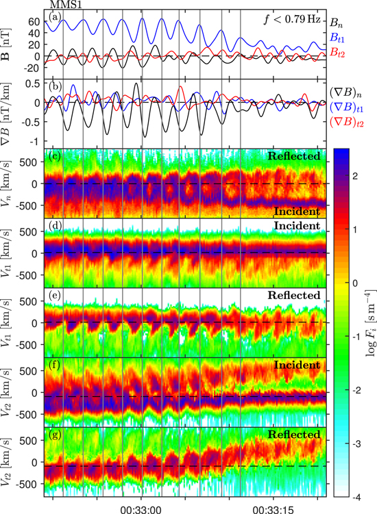
Figure 2. Magnetic field and ion phase-space density for MMS1. (a) Low-pass filtered magnetic field in shock aligned coordinates. Times where the B peaks are marked by vertical lines in all panels. (b) Gradient of B using measurements from all four MMS spacecraft. (c) The full ion distribution as a function of Vn measured by MMS1, integrated along the other two directions. The dashed line indicates the speed of the NI frame. The part of the distribution above the dashed line we call incident and the part above the line we call reflected. We use this simple separation for illustrative purposes only. (d)–(g) Partial ion distributions as a function of Vt1 and Vt2 showing the incident and reflected populations separately.
Download figure:
Standard image High-resolution imageWe also study the ion dynamics to investigate the non-stationarity mechanism. Figures 2(c)–(g) shows reduced ion phase-space density along the three principal velocity directions  ,
,  ,and
,and  . The ion phase-space density fi is integrated along the other two velocity directions so that
  . Panel (c) shows the full ion distribution as a function of Vn in the spacecraft frame. The speed of the NI frame
  is marked with a dashed line. In the following panels,we only show partial distributions corresponding to Vn < Vsh for incident ions and Vn > Vsh for reflected ions. We can make several important observations in figure 2. First,there are phase-space hole-like structures in Vn and periodic variability in the amount of reflected ions. Similar behavior is expected from simulations both of self-reformation (Lembège and Savoini 1992) and of ripples (McKean et al 1995). In both cases,the phase-space holes are due to the spacecraft periodically moving between the thermalized shocked downstream plasma and the upstream plasma,which is characterized by counter-streaming solar wind and shock reflected ion populations. Secondly,as can be seen in figure 2(d),the incident solar wind exhibits large fluctuations in Vt1. From the Rankine–Hugoniot relations (Landau and Lifshitz 1960),we find that the change in Vt1 from up- to downstream should be ∼10 km s−1. Any fluctuations arising from a change in shock strength (as in self-reformation) would be of this order. However,the observed fluctuations in Vt1 are >100 km s−1, clearly greater than expected for self-reformation. The Vt1 fluctuations can however be explained by local changes in
  due to shock ripples. To estimate the magnitude of the fluctuations from this effect, we assume the Rankine–Hugoniot relations are locally fulfilled in a rippled shock. This assumption is approximative since shock ripples is smaller than the fluid scales required for the Rankine–Hugoniot relations. We find that a relatively small turning of ∼10° in
  can explain the observed velocity fluctuations. Also the reflected ion velocity fluctuates greatly in Vt1, consistent with near-specular ion reflection of a shock surface that is periodically turning due to ripples. In figures 2(f)–(g) in the outbound shock foot, we can see the solar wind and reflected ions with large positive Vt2. Further downstream, the solar wind fluctuates in Vt2 due to a variability in the amount of reflected ions that together with the solar wind gyrate around the common center of momentum. The variability in reflected ions can clearly be seen in figure 2(g). A large portion of these reflected ions turn around before they reach upstream to the foot, see panel (f). Overall, the ion distribution functions in figure 2 support the case of non-stationarity in the form of shock ripples.
2.3. Dispersive properties
The ripples appear as quasi-periodic waves in the shock overshoot. Here, we determine the dispersive properties of these waves. The phase speed and direction of propagation,  is determined using timing analysis of low-pass filtered Bn from all four spacecraft. We use the timing method by Vogt et al (2011), which also gives error estimates of speed and propagation direction. Figure 3(a) shows Bn for all four MMS spacecraft as well as the time interval used in the timing. Figure 3(b) also shows Bn time-shifted so that the mean square deviation between the signals is minimized. The resulting phase speed in the spacecraft frame is 133 ± 12 km s−1 and
  in shock aligned coordinates (n, t1, t2) with an angular uncertainty of ∼7°. The timing shows that the waves propagate almost entirely in the coplanarity plane. The phase speed in the NI frame is 144 ± 23 km s−1 or
  , where
  is the local Alfvén speed in the overshoot. Furthermore, the angle between the local background magnetic field and propagation θkB is 42 ± 7°. In the spacecraft frame the frequency fSC is 0.46 ± 0.04 Hz, where the errors are the FWHM of the peak of the ripples in Fourier-space. In the NI frame, the frequency is
  or
or  . This yields a wavelength of λ = 290 ± 40 km or
  . Overall, the dispersive properties are in good agreement with those observed in 2D and 3D hybrid simulations (Lowe and Burgess 2003, Ofman and Gedalin 2013, Burgess et al 2016), and previous in situ observations, (Johlander et al 2016, Gingell et al 2017).
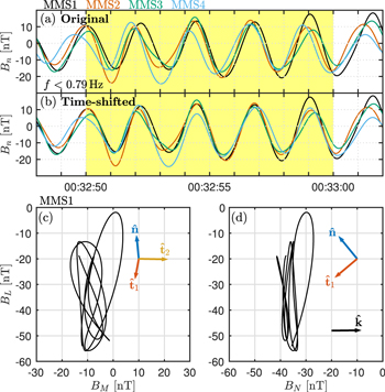
Figure 3. Results from timing and minimum variance analyzes. (a) Bn as a function of time for all four MMS spacecraft. The time interval used for both timing and minimum variance analyzes is indicated in yellow. (b) Bn for all four spacecraft but shifted in time to minimize the difference in signals. (c) B along intermediate and maximum variance vectors. (d) B along minimum and maximum variance vectors. The shock aligned coordinate system and  from timing is indicated in (c) and (d).
Download figure:
Standard image High-resolution imageThe observations show that the shock ripples propagate only in one direction. In our case the projection of wave vector is anti-parallel to an average magnetic field direction. In simulations, it is commonly observed that the waves propagate at the same time parallel and antiparallel to B (Lowe and Burgess 2003, Burgess et al 2016, Lee 2017). We note however that the simulations were performed with θBn close to 90° and that the smaller shock angle in the observations could be the cause for the symmetry breaking of wave propagation direction. In a recent simulation, Gingell et al (2017) observed shock ripples that propagated along B. However, in the simulations, the upstream magnetic field is pointing away from the shock,  , and one might therefore expect a different direction of propagation. What determines the preferred propagation direction remains an open question and requires further investigation.
The polarization of the ripples provides important information on magnetic structure and wave mode of the ripples. We therefore perform a minimum variance analysis (MVA) (Sonnerup and Scheible 1998) using the magnetic field. For the MVA, we use B measured by MMS1 in the time interval shown in figures 3(a), (b) band-pass filtered between 0.27 and 0.79 Hz. The resulting minimum variance vector,  , is within 10° from
  , in reasonable agreement with the timing analysis. It is also clear that the waves are nearly linearly polarized. Figures 3(c), (d) shows hodograms of B in the minimum N, intermediate M, and maximum L variance directions. The eigenvalue ratio between the maximum and intermediate variance vectors is ∼13. The direction of
  is nearly perpendicular to
  . These observations show that in addition to propagating in the coplanarity plane, the magnetic field fluctuations are also in this plane in the form of linearly polarized ripples.
2.4. Ion reflection off a rippled shock
Here, we in detail analyze how ion reflection depends on the phase of the ripples and on distance to the shock. In order to do this, we divide the shock into phase bins based on B fluctuations. Due to the quasi-periodic behavior of the waves, the phase bins are picked by hand based on the low-pass filtered B for each spacecraft. The phase φ = 0° is defined as the local maximum of B and φ = 180° as the local minimum of B . The bin width is set to 60°, and the rest of the bins are equally spaced between the 0°- and 180°-bins. The time intervals defined for all four spacecraft for every bin are shown in figure 4. After being divided into bins given the phase of the ripples, the data can be further divided into bins defined by the distance along the shock normal. We do this by assuming a constant overall motion of the shock in the normal direction. The time of an observation can then be transformed to distance from the shock. The width of these bins is set to 20 km. By assuming a constant wavelength of the ripples, we can further transform phase into tangential distance along the shock surface. This allows us to create maps of the shock in the  plane. An example of such a map is shown in figure 5(a) where the color denotes the average value of all measurements of B by any spacecraft in each bin. In the figure, the data is repeated two times side-by-side. Bins are slanted since the ripples propagate ∼40° downstream with respect to the shock surface. A constant wave phase φ then translates to a line
  . Also included in figure 5(a) are magnetic field lines constructed from the observed Bn and Bt1. For the field lines, we enforce
  while preserving the field as close as possible to the original. This does however mean that the Bn fluctuations are somewhat exaggerated in the field lines, likely due to the exclusion of Bt2. The magnetic field lines showing the structure of the ripples together with the maps of different physical parameters are helpful tools when analyzing the ripples.
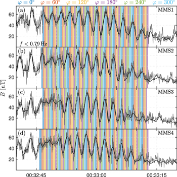
Figure 4. Magnetic field magnitude and the phase bins for all four MMS spacecraft. Full resolution B is shown as gray lines with the low-pass filtered B is overlaid as a black line. The phase bins for the individual spacecraft are shown as colored bars. The phase corresponding to the bin center for each bin is shown at the top.
Download figure:
Standard image High-resolution image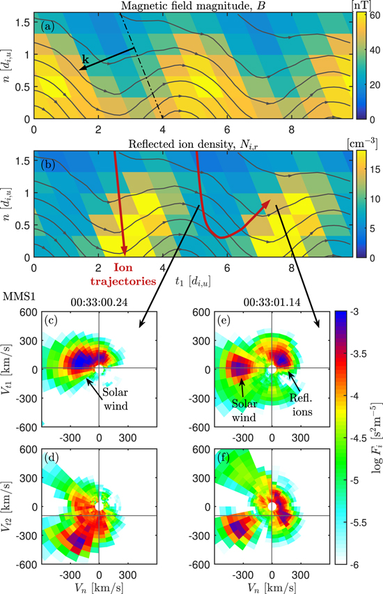
Figure 5. 2D histograms of the rippled shock compiled with data from all four spacecraft and representative ion distribution functions. (a) Magnetic field magnitude in the shock. Also shown are approximate field lines given from the magnetic field data. (b) Density of reflected ions. Two inferred ion trajectories for two incidence locations are shown as red arrows. (c)–(f) Projected ion distribution function, in two planes, for two times corresponding to different regions in the shock indicated by black arrows.
Download figure:
Standard image High-resolution imageNext, we investigate how ions are reflected in the shock. We have previously seen that ion reflection is highly variable in time. To determine how this translates to spatial variations we construct a map showing the density of ions that are moving upstream away from the shock,  . Most of the reflected ions after a gyration will be moving downstream towards the shock, which can be seen in figure 2(f) as incident ions with high positive values of Vt2. Thus,
  can be considered as the density of newly reflected ions that are between the point of reflection and the turnaround point. The map is shown in figure 5(b). The figure shows that the density of reflected ions is phased by the ripples and the highest density of reflected ions is observed in the region with the lowest magnetic field. Further upstream
  is displaced in the positive t1 direction. This is a clear indication that ion reflection is much more efficient in localized regions of the ripples.
The observed ion distribution functions indicate that ions are being reflected in regions of high B. Ion projections for two representative times are shown in figures 5(c)–(f). Here, Fi is the integrated phase-space density along the out-of-plane velocity component. The distribution in figures 5(c)–(d) is from a region with high B. Here, the solar wind is strongly heated and deflected and a part of the distribution has started to turn around to the upstream. The distribution in figures 5(e)–(f) is from a time with low B. Here instead the incoming solar wind is colder than in the previous case and less deflected. At the same time we see a relatively cold beam of reflected ions. The incoming solar wind and reflected populations are clearly separated in velocity space indicating that ion reflection is not occuring in this region. Instead, these ions were reflected in another part of the rippled shock because the reflected has positive Vt1 and that the ripples move in the negative t1-direction. We have drawn two approximate ion trajectories in figure 5(b) that explains the observed ion distributions. In the high-B region, the solar wind is slowed down and reflected. In the low-B region, the solar wind is relatively undisturbed, while at the same time ions reflected from the high-B region are observed here due to the motion of the ripples.
3. Discussion
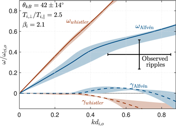
Shock ripples are often considered to be Alfvénic type waves. In simulation work, the shock ripples are often explained by the AIC instability by an ion temperature anisotropy (e.g. Winske and Quest 1988, Burgess et al 2016, Lee 2017). This reasoning is done by comparison between the simulation results and linear homogeneous theory. Here, we compare the in situ observations to wave modes from the numerical dispersion relation solver waves in homogeneous anisotropic magnetized plasma (WHAMP) (Rönnmark 1982). WHAMP does assume small amplitude waves in homogeneous plasma and in the setup we assume a single anisotropic Maxwellian ion distribution. These assumptions are unfulfilled for the non-linear ripples that propagate in the steep gradient of the shock ramp. This means that the results from this analysis should be considered approximative and can in the best case hint at the true nature of the waves. However, a more thorough theoretical description is outside the scope of this work. We use WHAMP to find dispersion relations for the Alfvén and the whistler branches in order to differentiate between the fluctuations observed in (e.g. Winske and Quest 1988) and (Hellinger et al 2007, Lembège et al 2009). The real and imaginary parts of the frequencies ω as a function wave number k for the two branches are shown in figure 6. For the calculations, we use plasma parameters measured by MMS in the overshoot and a propagation angle θkB = 42°. The dispersion relations show that the whistler mode is damped for these parameters while Alfvén waves have a positive growth rate due to the temperature anisotropy.
Figure 6. Dispersion relations for the lower and upper Alfvén wave mode from WHAMP and the observed ripples normalized to overshoot values. The solid lines show frequency and the dashed lines growth rate for the plasma parameters observed by MMS. Blue lines are for the Alfvén wave, red lines for the whistler branch. Error bars for the observations show the 2σ interval for k and ω and the shaded area show the 2σ interval for θkB. Uncertainties in the plasma and field measurements in the overshoot are omitted.
Download figure:
Standard image High-resolution image
We now compare the theoretical wave modes to the observed dispersive properties of the shock ripples. To further study the dispersive properties we need the wave properties in the local plasma (LP) frame, which is defined be averaged values of Vi in the overshoot. In the LP frame, the frequency is 0.29 ± 0.05 Hz and the phase speed is 82 ± 19 km s−1, see figure 6. Despite the caveats about nonlinearity and inhomogeneity, we note that the ripples closely resemble Alfvén waves. The ripples are observed at the wave number where the growth rate for AIC instability is positive. Furthermore, the observed frequency is a rather good match to that given by WHAMP for Alfvén waves. We also observe that the ripples are linearly polarized which is also the case for oblique Alfvén waves in WHAMP. For the observed plasma parameters, the whistler mode is damped. In addition, the frequency for whistler waves is higher and the observed waves are not clearly right-hand polarized as expected for whistler waves. The drift mirror mode has also been proposed as the source of the ripples (Winske and Quest 1988). We note however that drift waves typically propagate perpendicular to both the density gradient and B (Goldston and Rutherford 1995), opposite to what is observed here where the waves are propagating in the coplanarity plane. Other factors that could help us differentiate between mirror and Alfvén waves like B∥ fluctuations or compressibility are difficult to estimate due to the waves propagating in a strong gradient of magnetic field and density. We conclude that the ripples appear to fit the description of AIC waves although drift mirror waves cannot be entirely excluded.
When determining whether the shock was non-stationary due to ripples or self-reformation we made use of the Rankine–Hugoniot relations being locally fulfilled on the rippled shock. Such an assumption is approximative and requires validation. We can estimate the spatial amplitude of the ripples from figures 5(a), (b) or from the Bn fluctuations (Johlander et al 2016). In both cases we obtain a peak-to-peak amplitude A ∼ 30 km, or A/λ ∼ 0.1. If the ripples are sinusoidal in shape, this corresponds to a local change of  of at most ∼17°, in relatively good agreement with the ∼10° fluctuations required for the observed velocity fluctuations.
There are some questions about the shock ripples that this work does not answer. An open question about the shock ripples is that of direction of propagation. Here we find that the ripples propagate obliquely with a component anti-parallel to B, i.e. k · B < 0. Most simulations are done with nearly perpendicular shocks (e.g. Winske and Quest 1988, Burgess et al 2016) and the ripples there propagate both parallel and anti-parallel to B. A recent simulation by Gingell et al (2017) with θBn = 60° shows shock ripples propagating in the direction of B, contrary to the observations here. The difference in propagation direction can possibly be attributed to different sign of the upstream Bn, we observe Bn < 0, while the simulation has Bn > 0. The sign of Bn changes the guiding center motion of shock reflected ions in specular reflection (Schwartz et al 1983). It is possible this asymmetry could be linked to the propagation direction of the ripples. A detailed instability analysis taking into account the shock reflected ions is outside the scope of this study and is left for future work. Another open question is about the electron dynamics at the rippled shock. In simulations by Umeda et al (2009), shock ripples are associated with increased electron acceleration through shock surfing acceleration. The questions concerning direction of propagation and electron acceleration are left for future work.
4. Conclusions
We have studied one crossing by the MMS spacecraft of the Earth's quasi-perpendicular and non-stationary bow shock. During the crossing MMS graze the shock ramp and overshoot for an unusually long time. Magnetic field and plasma measurements on MMS show large fluctuation throughout the shock crossing, indicating that the shock is non-stationary. The slow crossing, combined with the favorable inter-spacecraft distances of ∼35 km, makes this event exceptionally well suited for studying ion-kinetic-scale fluctuations in the shock. Making use of multi-point observations and the high-cadence ion measurements, we conclude that the shock non-stationarity is in the form of ripples propagating along the shock surface.
The shock ripples are quasi-periodic fluctuations with a wave-like structure. Using timing and minimum variance analyzes, we accurately determined the dispersive properties of the ripples. We find that the ripples propagate in the coplanarity plane with an angle to the shock surface of ∼40° with k · B < 0 and  and with a phase speed in the NI frame close to the local Alfvén speed. The frequency of the ripples is ∼3 times the upstream ion gyrofrequency and the wavelength is ∼5 upstream ion inertial lengths. Moreover the ripples are nearly linearly polarized with fluctuations mainly in the coplanarity plane, leading to an almost two-dimensional structure of the ripples. Overall, these dispersive properties are in good agreement with 2D and 3D kinetic simulations (e.g. Lowe and Burgess 2003, Burgess et al 2016).
We compared the observations of the shock ripples with a numerical dispersion solver, assuming linear waves in a homogeneous medium. The assumptions of linearity and homogeneity might be invalid for the shock ramp. Despite this, the ripples resemble AIC waves generated by an ion temperature anisotropy.
Detailed analysis of ion dynamics dependency on wave phase and distance to the shock revealed that ion reflection is localized to regions of the shock with higher magnetic field. This shows that ripples play an important role in ion dynamics at shocks in space.
Acknowledgments
We thank the entire MMS team and instrument PIs for data access and support. For MMS data, see https://lasp.colorado.edu/mms/sdc/public/. The OMNI data were obtained from the GSFC/SPDF OMNIWeb interface at https://omniweb.gsfc.nasa.gov. This study was supported by Swedish National Space Board Contracts 139/12 and 97/13.