

Abstract
Infrequent, bursty, electromagnetic, whistler-mode wave packets, excited spontaneously in the laboratory by an electron beam from a hot cathode, appear transiently, each with a time duration  around ∼1 μs. The wave packets have a center frequency fW that is broadly distributed in the range 7 MHz < fW < 40 MHz. They are excited in a region with separate electrostatic (es) plasma oscillations at values of fhf, 200 MHz < fhf < 500 MHz, that are hypothesized to match eigenmode frequencies of an axially localized hf es field in a well-defined region attached to the cathode. Features of these es-eigenmodes that are studied include: the mode competition at times of transitions from one dominating es-eigenmode to another, the amplitude and spectral distribution of simultaneously occurring es-eigenmodes that do not lead to a transition, and the correlation of these features with the excitation of whistler mode waves. It is concluded that transient coupling of es-eigenmode pairs at fhf such that
  =
=  can explain both the transient lifetime and the frequency spectra of the whistler-mode wave packets (fW) as observed in lab. The generalization of the results to bursty whistler-mode excitation in space from electron beams, created on the high potential side of double layers, is discussed.
Export citation and abstract BibTeX RIS
1. Introduction and background
We report the continuation of laboratory studies of waves that are excited by electron beams in magnetized plasma. These studies are made to obtain better understanding of naturally occurring radiation from electron-beam-producing active regions in space plasmas. Three types of waves are found to dominate in our experiment: (1) localized electrostatic (es) oscillations at 300–500 MHz, sometimes in a narrow high-frequency (hf) spike structure that has been the subject of extensive earlier studies [1–4], (2) electromagnetic radiation, in the same range 300–500 MHz, which fills most of the vacuum tank, and (3) electromagnetic whistler mode radiation in the range 7–40 MHz appearing in 1 μs bursts, and with radiation patterns that depend on the specific frequency.
The properties of the whistler mode radiation were studied in detail in [5], herein called paper I. In the present work, we focus on the excitation of this whistler mode radiation. It is shown that the hf-spike Ez oscillations are composed of typically 2–8 discrete es eigenmodes, temporally overlapping and each typically of 0.2–2 μs duration. Their spectral development in time falls into two categories: slow frequency-drifting of individual es-eigenmodes, typically Δf/f = 2%–5%, per μs, and fast frequency-transitioning, or frequency-jumping, of 30 MHz < Δf < 60 MHz in which one dominating es-eigenmode is replaced by another. Always, including during such transition times, there is, in the proximity of the dominating es-eigenmode frequency, a 'void gap' in which secondary es-eigenmodes are absent. This void gap is in the range ±5 to ±40 MHz, and increases with the amplitude of the dominating es-eigenmode. This is a central finding for the excitation of whistler mode radiation, which is found to require the simultaneous presence of two es-eigenmodes of significant amplitude over numerous wave periods of the es-eigenmodes, meeting a frequency matching condition that  This transient coupling of pairs of es-eigenmodes, interpreted as periodic frequency-and-wavelength pulling [6] during mode competition [7], explains the transient lifetimes, and also the spectral distributions, of whistler-mode wave packets fW as reported in paper I.
This paper is organized as follows. In section 2 the apparatus and the diagnostics are described. Section 3 contains experimental data on the hf-spike Ez oscillations, focusing on their spectrum in terms of es-eigenmode identification. In section 4, this is combined with measured whistler mode data to identify the excitation mechanism of whistler mode radiation. Section 5 treats whistler mode emission by an electron beam that is created by a double layer, and not by a cathode sheath as in the present experiments. Section 6 consists of a summary and discussion.
2. Apparatus and diagnostics
Figure 1 is a schematic diagram of the Green tank [1], in which the experiments reported here are performed, and the diagnostic-probe [5, 8] arrangement in it. The Green tank is operated in a cathode-sheath configuration that was also used in several of the previous studies of the hf-Ez oscillations [9–11]. Electrons from the hot cathode stream into ambient plasma (ne ≈ 1015 m−3) along the axial direction as defined by the magnetic field produced by a multi-turn coil concentric with the cathode. Over a region having an axial dimension of (0.025 ± 0.005) m starting at the cathode, the cathode sheath potential USH can be adjusted within the range 35–210 V by controlling the applied voltage U, in response to which the electrons are accelerated to form a beam.

Figure 1. The Green tank in which the experiments are made. The cathode, anode ring, floating plate, and hf-region are described in the text in terms of plasma production.
Download figure:
Standard image High-resolution imageThe magnetic field strength is 2.6 mT at the cathode and decreases with increasing z along the central axis as indicated by the diverging field lines. Inside the radius given by the magnetic field lines that map to the edge of the cathode, there is a core of high-temperature (5 eV < Te < 10 eV) plasma, which also contains a fraction of the beam of electrons. Here, we limit the investigation to a standard discharge, also used in paper I, with parameters:  mbar,
mbar,  A, and
  V. The probes used for measuring the wave electric and magnetic fields are tailor-made for these studies, but are designed based on earlier probe constructions that have been developed in our laboratory and are reported elsewhere [12, 13].
The anode ring (biased +57 V from the chamber) surrounding the cathode (−75 V biased from the chamber) has an outer diameter of 33 cm and an inner diameter of 10 cm. The anode–cathode current is 0.6 A. The cathode is indirectly heated by hot, electron-emitting, negatively biased, tungsten filaments directly behind the cathode plate.
An electron beam is emitted, in the uniform-field region of the magnetic mirror, from the heated (1500 °C) LaB6 cathode of diameter 3.5 cm, also negatively biased, and enters the plasma along the magnetic field. Some electrons from the cathode must move across the magnetic field to reach the anode ring and the plasma is formed between the cathode–anode plane and a metal plate, at (negative) floating potential, placed 60 cm from the cathode. In combination, the cross-field electron motion and field-aligned electron beaming produce the plasma.
The electron beam, from the negatively biased, LaB6, hot cathode of diameter 3.5 cm, enters the plasma, and it leaves the magnetic mirror along the magnetic field. Most of the applied voltage is concentrated in a cathode sheath. The beam current and the beam energy can be varied in the ranges I = 0.2–1 A, and eUSH = 65–130 eV, here we apply 0.4 A and 122 eV. The beam's thermal spread is 10 eV and the electron gyroradius is 1 mm in the cathode–anode gap where electrons undergo many gyrocycles while E × B drifting azimuthally.
The small hatched box bordered by thick dashed lines in figure 1 represents the region where the electron beam loses its beam character by interaction with the plasma, and where the hf-Ez oscillations are found. The axial extent of this HF region varies slightly as a function of the applied voltage U [3]. For the experiments reported here, the HF region starts approximately 5 cm from the cathode, extends approximately 7 cm along the cylindrical axis, and supports a density gradient having a scale length of approximately one cm and a parallel electric field of approximately 5 kV m−1. A short-interaction-length mechanism is responsible for scattering of the beam in this HF region by waves and es structures [3, 14]. We have identified this region as the source for the whistler mode radiation. We regard this region also as the most likely source for the electromagnetic radiation. The scattered beam electrons magnetically map as a flux tube that approximately matches the floating plate. The beam density is about 25% of the total electron number density. The beam density was calculated from the measured current and the velocity gained from the acceleration in the cathode sheath [2].
3. Hf es eigenmodes
3.1. Preamble regarding the new mechanism evidenced by the copious generation of transient whistler wave packets from a dc discharge
Extended earlier studies of the hf-Ez oscillations were made in the late 1990s by Gunell, Löfgren, and co-workers. They used the Green tank in two different configurations—first as a double layer device [1] and later [2, 3] in the cathode-sheath configuration also used here. They identified as a key feature in both configurations that a dense and suprathermal electron beam enters a region with increasing plasma density [3]. When the beam enters the plasma, it drives high-amplitude, hf, es oscillations, 200–500 MHz, with Ez up to 9.3 kV m−1 [3] in a spatially localized 'hf-region', with highest amplitude typically (0.05 ± 0.02) m from the cathode and within the plasma-density-gradient region found there. These oscillations were extensively studied earlier [1–3] and will be referred to as hf-Ez oscillations. In these earlier studies, the axial hf es-field profile and its frequency were found to have the same variability in time, on time scales typically 1 μs. In most of these earlier studies, the focus was on the occasional appearance of a high amplitude 'hf-spike' with very short spatial extent, e.g., a few Debye lengths. The spatial and temporal wave pattern of this hf-spike was studied in detail, including duplications of experimental wave data by simulations [3]. It was identified as a region having a high-amplitude standing wave surrounded by regions having lower-amplitude, overlapping, backward- and forward-traveling waves. The solid curve in figure 2 shows the maximum hf-Ez amplitude as function of location along the z axis, while the data below the curve shows the spatial profile of one example of a hf-spike, in this case centered at z = 0.05 m. This hf-spike profile was recorded with an Ez-probe array, and with the sampling conditions that the amplitude at 0.05 m is close to 2 kV and also nearly steady in time [3].
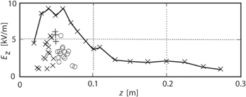
Figure 2. Electrostatic hf-Ez wave data from [3] for a 95 V cathode sheath. The solid curve connects the maximum amplitudes as function of distance from the cathode, showing a 0.1 m extent of the hf-region. The data points below the curve are obtained by conditional sampling, and show the spatial profile of a hf-spike centered at z = 0.05 m.
Download figure:
Standard image High-resolution imageThe hf-spike, however, is not the typical hf-Ez wave pattern. The amplitude of the oscillations varies considerably within the hf-region, on typical ion acoustic time scales 0.5–1 μs. Sometimes the wave pattern is spread out, having lower amplitude, and, at other times, it is more concentrated and having higher amplitude. From a combination of experiments, particle-in-cell simulations, and an analytical fluid description [4], the hf-Ez oscillations were understood to be a family of discrete es eigenmodes of the system. We will herein call these 'es-eigenmodes'. In an experimental case where a hf-spike was produced, two strong es-eigenmodes with the harmonic relation  were identified, and an interaction between these in the creation of the hf-spike was tentatively proposed [4]. Although the hf-spike case, on which these earlier studies was concentrated, does not generally create the highest amplitudes of whistler mode emission, we have found to be central their analysis of the data in terms of discrete es-eigenmodes.
There is an extensive literature (see e.g. [10] and references therein) on whistler mode excitation by antennas, by pulsed currents, and by electron beams. Some proposed mechanisms for electron beam excitation [15–17] were briefly discussed in paper I [5]. None of those mechanisms apply here. Instead, the whistler mode excitation mechanism reported here has the following features.
- A whistler mode wave can be excited when, besides the dominating es-eigenmode, there is a secondary es-eigenmode with significant amplitude, approximately
 and with a frequency such that Furthermore, this frequency must fall in the range
- When these conditions on amplitude and frequency of the two es-eigenmodes are met, a whistler almost always results. The whistler mode phase velocity is low enough to allow wavelength matching and the whistlers are close to es in nature, which allows coupling to the es-eigenmodes.
- Because of temporal variations of the es-eigenmode spectrum of the hf-Ez oscillations, only seldom are both the conditions above on frequency and amplitude met and, only then, a whistler mode burst almost always results.
- Both high- and low-amplitude whistler wave packets originate from the same source region, the smaller hf-region, see e.g. Figure 1, in which the hf-Ez oscillations are found.


3.2. Amplitude distribution and time duration of the es-eigenmodes
Figure 3 shows an example of analysis of hf-Ez data, in this case specifically selected for a rich content of es-eigenmodes. The top panel shows the time series, and the middle panel shows the fast Fourier-transform (fft) amplitude obtained with a moving time window of 0.2 μs length, giving a spectral resolution of 5 MHz. The spectrum is seen to be composed of discrete peaks, each of which appears briefly, remains close to the same frequency, and then disappears. We identify these peaks as the es-eigenmodes of Gunell and Löfgren [4]. The bottom panel shows a way to represent the fft data that we have found useful for analyzing the whistler emission process: the 'fft peak plot'. In this case it includes all the peaks in the fft that can be clearly identified above the noise level.
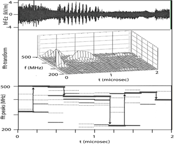
Figure 3. An example hf-Ez data. The top panel shows the time series of the hf-Ez field on the axis, at z = 0.0 m. The second panel shows fft spectra, and the third panel, a 'fft peak plot', depicting the spectral locations of the peaks in the fft. In this, the three strongest peaks are drawn with solid lines of decreasing width, and all the weaker peaks with dashed lines. The vertical arrows show the times when the dominating es-eigenmode is replaced by another at a different frequency.
Download figure:
Standard image High-resolution imageFor the amplitude distribution of the es-eigenmodes in typical data, i.e., that has not been selected for e.g. hf-spike or whistler emission, we have made a spectral analysis, such as shown in figure 3, of 50 consecutive random-triggered recordings, 2 μs long, of hf-Ez in the middle of the hf-region, at z = 0.035 m. In that data, the hf-Ez amplitude was always between 0.3 and 4 kV m−1, and clearly above the noise level. At each given time, typically 2–8 simultaneous es-eigenmodes were possible to identify. Usually the strongest es-eigenmode has much higher amplitude than the others, and therefore will be called the dominating mode. For a quantitative analysis, we denote the dominating es-eigenmodes' amplitude as A1 at a frequency f1, the next amplitude is denoted A2 at f2, and so on. For about 75% of the time the dominating mode has an amplitude more than ten times that of the second strongest mode, i.e.  Around 75% of all the observed secondary es-eigenmodes are below 1% in power of the strongest. Cases of two or more relatively strong es-eigenmodes of comparable amplitude (here defined as
  ) are only found 10%–15% of the total time, and are almost always associated with transitions from one dominating es-eigenmode to the next.
Now, let us have a look at the time duration of the es-eigenmodes. Typical time durations can be seen in figure 4. In order not to introduce any bias in the selection, we have chosen the first 9 consecutive recordings in our 50-shot random triggered data set. In figure 4, there are 15 total dominating-mode transitions during the combined 18 μs, giving an average length of 1.2 μs. In the full 50-shot data set, dominating modes have average time duration 1.5 μs, and only a few percent of them are shorter than 0.6 μs. Generally, the secondary modes last shorter, lasting, typically, less than 0.6 μs, as short as the limit 0.2 μs set by the fft time resolution, and appear both at and inbetween dominating-mode-transition events.

Figure 4. Nine fft peak plots from random-triggered hf-Ez data, here showing only the three strongest es-eigenmodes. Transitions from one dominating es-eigenmode to the next are marked by arrows, and numbered T1—T15.
Download figure:
Standard image High-resolution image3.3. Frequency-domain features of the es-eigenmodes
In the frequency domain, we have made statistical and overview studies of the es-eigenmodes based on three observables, namely, the drift in frequency during their lifetimes, the occurrence of a dominating-mode transition, and the distribution of frequency differences between simultaneously occurring es-eigenmodes.
A first estimate of the frequency drift can be obtained from fft peak data, as shown in figure 4. This yields a typical drift of 10–20 MHz, or 2%–5% during the 1 μs lifetime of a typical dominating es-eigenmode at 400 MHz. The relative frequency drift in a wave period is only of the order of (df/dt)/f2 = 0.01%. One disadvantage with Fourier transform data such as figures 3 and 4, however, is the trade-off between time resolution and frequency resolution. The fft cannot resolve whether this drift is continuous or is a compilation of a sequence of small discrete transitions. As seen in section 4, below, the difference between continuous or discrete drifting is an important issue to resolve since transitions are associated with times of mode competition that can give rise to whistler-mode wave emission. In the cases having usually one dominant frequency, as we have here, the instantaneous-frequency method [6, 7] makes it possible to improve the combined time- and frequency resolutions, but at the cost of losing the oscillation amplitude information. The 'instantaneous frequency'  is obtained from the time
  between every second zero crossing, where zero crossing refers to the time at which the oscillating signal crosses the signal's locally averaged value. Choosing such pairs of zero crossings reduces systematic artifacts in the representation of frequency modulation from non-sinusoidal signals. The array of zero-crossing periods is converted to an array of instantaneous frequency using the simple relationship
  Special care must be taken in the analysis when more than one additional spectral component is present besides the dominating one. Such a case is shown in figure 5(c), using the same hf-Ez data as in figure 3 that has a rich content of es-eigenmodes. The presence of many simultaneous modes destroys the simple identification of the dominating mode. However, a detailed comparison between figures 3 and 5(c) reveals that the lower boundary to the
  -frequency, even during noisy time intervals, often coincides with the dominating es-eigenmode in the fft peak plot. When only two modes are present the analysis is somewhat simpler. As long as
  there is an oscillation of the
  value around the frequency of the dominating mode,
  with an oscillation amplitude that is approximately proportional to
  and an oscillation frequency
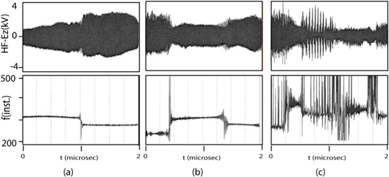
Figure 5. Top: time series of hf-Ez. Bottom: the instantaneous frequency  obtained from the data in the top panels. (a) and (b) are from typical random-triggered recordings, while (c) uses the same data as figure 3, with a rich content of es-eigenmodes.
Download figure:
Standard image High-resolution imageFigures 5(a) and (b) shows hf-Ez time series and  -plots from two typical cases where there are only low amplitude secondary modes. There are three mode transitions, with jumps in frequency of 30–60 MHz. Modulations of the 'two-mode' kind are seen around the transition of figure 5(a), and at the second transition in figure 5(b). If the slow drifts between these three transitions contained smaller transitions, these would be revealed by two-mode oscillations during the times when the two involved es-eigenmodes are present, we have found no case of that anywhere in the data set. In summary: the frequency changes, except a 0.2% minority of uncertain cases, fall into one of two categories. The most usual category consists slow changes with a typical value of
  MHz μs−1, but always in the range
  MHz μs−1. These are continuous drifts of existing dominating es-eigenmodes. The minority category consists of more rapid frequency changes,
  MHz μs−1, and are transitions from one to another dominating es-eigenmode.
The most interesting es-eigenmode transitions here are those with small frequency jumps, below the electron gyro frequency  MHz, which we have found (see section 4 below) can be directly correlated to whistler mode wave emission. The frequency jumps of the 15 transitions in figure 4 all lie above 35 MHz. This is quite typical; in the whole 50 shot random-triggered data set, only 7% of all transitions are below 40 MHz. The time durations of the transitions are also of interest. We define these as the time during which the two involved es-eigenmodes are simultaneously present. A typical value, from the fft peak plots, is 0.2–0.4 μs, but sometimes the transition time extends up 0.6 or even 0.8 μs. About 50% of the transitions are abrupt in the sense that one mode is more than ten times the spectral amplitude than the other, and within the time resolution of the fft, 0.2 μs, the amplitude relation becomes reversed. Examples of such abrupt transitions in figure 4 are numbered T1, T2, T4, T6, and T13. The
  data can be used to obtain even better time resolution. An inspection of the full data set shows that the duration of mode competition at transitions, as revealed by two-mode modulations in the
  data, can be as short as ∼50 ns.
The final aspect of the es-eigenmode spectra is the distribution of frequency differences between the dominating mode and simultaneously occurring secondary modes. We exclude from this study secondary es-eigenmodes that are 2nd or 3rd harmonics of dominating modes at lower frequency. They number about ¼ of all secondary modes. They might be involved in the hf-spike process as proposed by [4], but we have found them not to be correlated to whistler-mode wave emission. Figure 6 shows the relation between the amplitude  of the dominating mode at
  and the frequency differences to all secondary modes during the same time interval, i.e.
  The near frequency surroundings around the dominating mode is found to be surrounded by a region with a lower number of secondary es-eigenmodes, and in the center of this region there is a gap in frequency where secondary modes are completely absent. This gap increases with the amplitude of the dominating es-eigenmode. Let us call this the 'mode void'. We have checked that the mode void is not an artifact in the sense that the dominating modes are so broad in frequency that weaker modes
  on the flanks would disappear. As an example, secondary es-eigenmodes down to
  would have been possible to resolve as close as ±6 MHz from the strongest dominating es-eigenmode in our whole data set. Since the mode void is much wider than this, ±30 MHz for high amplitudes, we conclude that it is real, and casually connected to the presence of the dominating mode. As we shall see below, the mode void strongly counteracts the mechanism of whistler mode wave excitation. To understand the mode void therefore is a key problem for the scaling of whistler mode excitation efficiencies to space, and also for the understanding of the experimentally determined scalings with power and electron beam energy reported in [5]. This falls outside the scope of the present study, but we note that the mode void might be related to Arnold tongues [18], regions in the frequency domain from which weaker eigenmodes are absent because they are entrained by stronger modes.
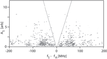
Figure 6. The distribution of frequency differences between dominating and secondary es-eigenmodes, from random-triggered fft spectra of hf-Ez over time windows of 0.2 μs length. The plot shows the amplitude  of the dominating mode at
  versus the frequency differences to all secondary modes during the same time interval, i.e.
Download figure:
Standard image High-resolution image4. The relationship between es eigenmodes and whistlers
In paper I [5], detailed studies were made of whistler mode waves in the bulk plasma, outside of the hf-region. They were found to appear in the form of bursts, or wave packets, each with typically 0.1–1 µs time duration, and together covering typically a few percent of the full time. Such wave packets were found in a broad frequency range of 7–40 MHz, but each individual wave packet usually was dominated by a single frequency. Averaged over many wave packets, the dominating frequency at each location decreases with increasing z at the same rate as the magnetic field decreases, so that the maximum of the spectrum everywhere lies in the range 50%–80% of the local electron gyro frequency. Ray tracing showed them to come from a source region in the central channel of the device, around  m, and
  to
to  m. From this source region, they propagated into the ambient plasma along two routes, as exemplified in figure 7. One propagation path was at the group velocity resonance cone angle
  to the magnetic field [10]. This gives wavefronts that curve away from the central axis as seen in figure 7, and also exemplified in figure 1 for 16, 20, and 26 MHz. The other channel consists of central waves. These decrease in amplitude for increasing z, probably because in the decreasing magnetic field gyro resonance is approached. Features of the whistler mode wave packets that were studied in paper I include the statistics of amplitudes, frequencies, and time durations, the propagation and decay of wave packets with different frequencies, the group and phase velocities, and how the wave packet production varies with the energy, and the current density, in the electron beam.

Figure 7. The time-averaged signal level of whistler mode wave packets at 14.5 MHz, obtained by narrow band-pass filtering, reproduced with permission from [5]. The 'wings' to the side are consistent with propagation along the group velocity resonance cone angle at the selected frequency.
Download figure:
Standard image High-resolution imageIn the present paper II, we focus on the excitation of these whistler mode waves by the hf-Ez oscillations. In view of the high variability of both the hf-Ez oscillations and the whistler mode wave packets, some constraints in parameter space are needed. In addition to using the standard discharge parameters  mbar,
mbar,  A, and
  V, we make a closer study only of 20 MHz whistlers. These were found in paper I to be in the central range, both in frequency and in the spatial distribution. They are monitored by a magnetic pickup coil placed at
 m, on the 20 MHz resonance cone. This is the '20 MHz
  -coil' shown in figure 1. When we use random-triggered data, this probe will act as a frequency bandpass filter. Out of a broader range of excited whistlers, it will with highest sensitivity record those with close to 20 MHz, but also pick up the lower amplitude fringes of larger wave packets at nearby frequencies, that are centered at close lying resonance cones. Data collection triggered on the 20 MHz
  -coil, on the other hand, will select cases of excitation where wave packets around that frequency are created. It is important to remember, however, that the dominance of 20 MHz in the data of the present paper is only a consequence of these two types of selection. Whistlers in the full range 7–40 MHz are created, but usually not recorded. We have separately ascertained that their excitation has the same main characteristics as that being reported below for the 20 MHz whistlers.
4.1. Typical whistler emissions
The typical 20 MHz whistler emission features can be exemplified by data from the nine random-triggered recordings shown in figure 4. In this data set, we found only two clear cases of whistlers at the 20 MHz  -coil, and both of them only medium sized. They are shown in figure 8(c). The whistler emission periods are the first 0.3 μs of shot #5, and the last 0.2 μs of shot #6, together only 3% of the total time of the nine recordings in figure 4. This is a demonstration of the rarity of whistlers, particularly of high amplitude, and consistent with the findings in paper I. The fft peak plot in figure 8(b) gives a first clue to the reason for this rarity: at the times of whistler emissions, the two strongest es-eigenmodes have a frequency difference
  MHz that matches the whistler frequency. As demonstrated in figure 6 this is an unusually small frequency difference, and particularly so for cases with a strong dominating es-eigenmode. In all of the fft peak data of figure 4, we find only three time intervals when
  MHz . Only one of them, at 1.5 μs in shot 5 of figure 4, failed to give a clear whistler signal on the 20 MHz
  -coil. (It could be noted here that we cannot exclude the possibility that a whistler is emitted in another azimuthal direction, although paper I indicated that at least large amplitude whistlers are emitted quite isotropically.) This means that there are strong correlations both ways: whenever there is a 20 MH whistler, there are es-eigenmodes with that frequency difference, and whenever there is such a pair of es-eigenmodes, a 20 MHz whistler is almost certain to be produced. We have checked that these conclusions hold also for a larger data set of 50 random triggered and 50 whistler triggered recordings.

Figure 8. Data for the only two whistler mode wave packets that were produced during the nine random-triggered recordings shown in figure 4. (a) The time series of the hf-Ez signal. (b) The fft peak plots, also shown in figure 4. (c) The signal from the 20 MHz  -coil. The two whistler mode wave packets have 20% and 10% of the peak whistler amplitude, respectively.
Download figure:
Standard image High-resolution image4.2. Large amplitude whistler emission
It was demonstrated in paper I [5] that the highest amplitude whistler wave packets are very rare events. Figure 9(c) shows three cases of such unusually strong whistlers, here triggered at 70% of the maximum amplitude recorded on the 20 MHz  -coil. Figure 9(b) shows the fft peak plots. At the times of whistler mode emission, they are seen to depart dramatically in two ways from the random triggered examples of figure 4. First, there is always at least one competing mode with ∼20 MHz difference from the dominating mode; such a small frequency difference is only found in ∼3% of the random triggered recordings. Second (from data not shown here), the secondary es-eigenmode amplitude, at the time when the whistler emission peaks, is at least 10% of the dominating mode; this is the case in only 25% of the random triggered recordings. Thus, there are two conditions on the es-eigenmodes to produce a high amplitude whistler: an amplitude
  of a secondary es-eigenmode, and a frequency matching such that
  We can note that the earlier-shown figure 3 fulfills both conditions from 0.6 to 1.2 μs, and that a large a 20 MHz whistler mode was indeed emitted.

Figure 9. Three examples of strong whistler emission, here from recordings triggered at 70% of the maximum whistler amplitude. (a) The hf-Ez time series at  m. (b) Corresponding fft peak plots. (c) The signal from the 20 MHz
  -coil.
Download figure:
Standard image High-resolution imageThe cases in figure 9 were selected to show two features that are often seen. First, large amplitude whistlers are almost always within 0.2–0.4 μs of dominating-mode transitions, but only seldom does the transition jump in frequency match the whistler frequency. Instead a third mode appears and disappears, and the whistler is emitted only during its lifetime. Second, the two es-eigenmodes that give the whistler mode emission can drift in relative frequency. This drift, e.g. from 20 to 25 MHz in the third recording in figure 9, is then reflected in the whistler frequency.
Figure 10 shows a very unusual case, selected out of the recordings triggered on the 20 MHz  -coil: a mode transition between two es-eigenmodes of comparable amplitude, and with
  20 MHz. The two modes compete for 0.4 μs before the transition is completed and, during that time, a 20 MHz whistler is emitted. Panel 10(b) shows the hf-Ez field on the central axis. The beat, 'herringbone', frequency that is apparent as an amplitude modulation agrees with the whistler-mode frequency in panel 10(a),
  20 MHz. It is understood as a beating between a pair of waves where
  Spectra before and after the amplitude modulation event (rightmost and leftmost panels of figure 10(c)) show that whistler-mode excitation occurs only during the period within which the two interacting eigenmodes are present simultaneously. The time delay (0.1 μs < time delay < 0.2 μs) associated with the whistler-mode appearance and disappearance with respect to the hf-Ez amplitude modulation, is consistent with the whistler-mode propagation time from the source region to the magnetic probe location, with the group velocity of the order of 106 m s−1 measured in [5].
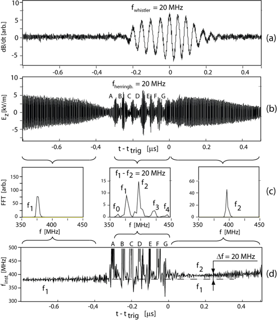
Figure 10. A selected case of a mode transition with a dominating-mode frequency jump of 20 MHz, and a matching whistler mode emission. (a) The signal from the 20 MHz  -coil, that was used for triggering of this event. (b) The signal on the central axis, at
 (c) Fourier spectra of hf-Ez over the indicated time intervals. (d) The instantaneous frequency
  obtained from the hf-Ez data in panel (b).
Download figure:
Standard image High-resolution image4.3. Probe array measurements
All data presented so far are from measurements with only two probes: one hf-Ez probe at  =
=  and the 20 MHz
  coil at
  =
=  This does not adequately reflect the time and space variations of the mechanisms we study. Figure 11 shows two examples of recordings with four-probe arrays, spread out in the z direction, of both hf-Ez and
  Detailed study of this type of data falls outside the scope of this paper, but we will make a few interpretive observations.
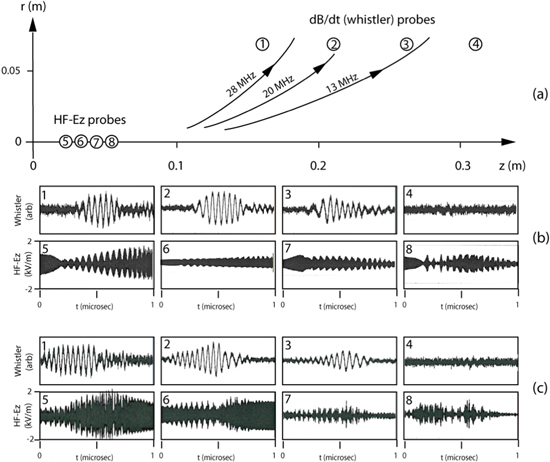
Figure 11. Spatial and temporal distributions of the  (whistler) and the hf-Ez oscillations, from two simultaneous multi-probe measurements (b) and (c), both triggered on high amplitude of the
  probe no 2. Probes 1–4 are at (
 z = 0.17, 0.22, 0.27, 0.32), and probes 5–9 at (
 z = 0.025, 0.035, 0.045, 0.055).
Download figure:
Standard image High-resolution imageThe whistler signal on probes 1–4 can be understood as whistler mode radiation that propagates, depending on its frequency, along the resonance cones as indicated in panel 11(a). Fourier transforms (not shown here) of the whistler signals in panels (b1) and (b2) show that the signals have very close to the same frequency, 19.7 MHz. This indicates that one whistler mode wave packet crosses both probes 1 and 2, and therefore has at least 0.04 m extent in the z direction. Probe 3 at a higher z coordinate shows a slightly lower frequency, 18.6 MHz. In the second example (panels (c1)–(c8)), probe 1 shows a 21.5 MHz whistler up to 0.5 μs, which during that time has high amplitude on the neighboring probe 2, much lower amplitude on probe 3, and is absent on probe 4. Around 0.5 μs the frequency decreases to 16.7 MHz and the radiation changes propagation path: it disappears on probe 1 and is now seen mainly on probes 2 and 3, but also with very low amplitude on probe 4.
The four hf-Ez signals, from probes 5–8, show complicated spatial, temporal, and frequency variations with typical timescales below, or around, 1 μs. We will not explain these further; we only note that already [1–3] reported that such a high variability is characteristic for the hf-regions, both in the cathode-sheath and the double layer configurations.
5. Whistler emission mechanism
In contrast to the extensive literature on whistler mode excitation, a new mechanism with the following features is the only mechanism applicable in our experiment.
- A whistler mode wave can be excited when, besides the dominating es-eigenmode, there is a secondary es-eigenmode with significant amplitude, approximately and with a frequency such that Furthermore, this frequency must fall in the range This indicates wave-wave coupling involving two es-eigenmodes that interact to produce the whistler mode, and obeying the frequency matching condition
- When these conditions on amplitude and frequency of the two es-eigenmodes are met, a whistler almost always results. The plasma thus seems to be able to, almost always, find a whistler mode that satisfies also the propagation constant (k) matching condition Both the wavelengths and the orientations of the k vectors must match. We discuss this in appendix and conclude that k matching is why whistler mode radiation is seen to follow the resonance cone. Therefore, the whistler mode phase velocity is low enough to allow wavelength matching and the whistlers are close to es in nature, which allows coupling to the es-eigenmodes.
- In spite of the continuous presence of both the energy source (the electron beam) and the exciting agent (the hf-Ez oscillations), whistler modes waves are usually not excited, and then only appear in short bursts or wave packets. The reason is now identified as the temporal variations of the es-eigenmode spectrum of the hf-Ez oscillations. Only seldom are both the conditions above on frequency and amplitude met, and then a whistler mode burst almost always results.
- Ray-tracing in paper I indicated that both high- and low-amplitude whistler wave packets came from the same source region, somewhere around z = 0.05–0.2 m. This can now be narrowed down to the smaller hf-region, see e.g. figure 1, in which the hf-Ez oscillations are found. Within this region, the whistler source probably varies in axial extent, and also moves back and forth, following variations of the hf-Ez time and space distribution such as exemplified in figure 11.


6. Whistler mode emission from double layers?
As discussed in paper I, a major motivation for these studies is to obtain better understanding of naturally occurring radiation from electron-beam producing processes in space plasmas. Of particular interest, here, are electric double layers, DL's [2, 3, 19, 20]. These are current-carrying plasma structures in which strong local electric fields can be sustained within a limited region of space, producing current-dense electron beams on the high potential side. The first studies of hf-Ez oscillations in our laboratory were made at double layers: first in the Green tank [1] and, slightly later, in a triple plasma device [21]. In both configurations, the electron beams were found to drive hf-Ez oscillations with the same characteristics as in the cathode-sheath configuration used here: field strengths of a few kV/m, a time and space variability on a μs time scale, time-averaged frequency spectra a few 100 MHz wide around the local plasma frequency, and a wave phase velocity slightly below the electron beam velocity.
In view of these similarities, we regard it as likely that also the DL-associated hf-Ez regions give emission of whistlers. A direct indication for this to be the case is that herring-bone patterns, demonstrated in section 3 to be strongly correlated with whistler mode emission, were seen in both these double layer experiments. Figure 12 compares hf-Ez time series from the three experiments. Panel 12(a) is from our cathode-sheath configuration, an extract from the 2 μs long recording in figure 3(a). The herring-bone pattern (see figure 3(c)) is here produced by the beat between two competing es-eigenmodes at  MHz and f2 = 400 MHz. Simultaneously, and only during that time, a whistler (not shown here) was measured by a
  pickup probe. The frequencies are related by
  =
=  MHz. As required for whistler mode waves, when
  as in the Green tank, this is below
  ≈ 35 MHz at the location of the probe.

Figure 12. Herring-bone patterns of hf-Ez oscillations measured in three experiments. (a) From the present experiment with the Green tank in the 70 V cathode-sheath configuration. (b) From the Green tank operated in a 27 V double-layer configuration, from [1]. (c) From a 50 V double-layer experiment in a triple plasma device [20].
Download figure:
Standard image High-resolution image
Panel 12(b) shows a very similar hf-Ez time series from the Green tank in the double layer configuration from [G2] (notice the different time scale). Here  MHz, again in the whistler mode range below
  here
here  MHz. By analogy to panel 12(a), we propose that a whistler is likely to have been excited also here, although there was no diagnostic to measure it.
The double layer experiment by Ljungberg [21] differed in several respects. The magnetic field was homogeneous, and the plasma was produced in a triple plasma device with two plasma sources that were geometrically separated from a central chamber where the double layer was formed. These experiments were in a lower plasma density so that  which has important consequences for whistler mode radiation; among else, it requires
  In spite of these differences, also here herring-bone patterns were produced: panel 12(c) shows a hf-Ez time series with
  MHz. Although this is further below
  (here,
  ∼ = 280 MHz) than in the other two cases, it is also here in the right frequency range for whistler emission.
7. Summary and discussion
It was shown in paper I that regions of dense electron beams in laboratory plasmas can copiously produce transient bursts of electromagnetic whistler-mode wave packets. The mechanism is here identified as the production, by the electron beam, of hf-Ez oscillations that are spread out spectrally over a few 100 MHz around the local plasma frequency, and composed of short-lived (time duration of 0.2–2 μs) eigenmodes of es Langmuir waves. Usually one such es-eigenmode is dominating while a number of secondary modes of lower amplitude are also present. Equally transient (typical time durations 0.4–1 μs) electromagnetic whistler-wave packets are produced when there is at least one secondary mode to which there is a mode-difference frequency, relative to the dominating mode, in the whistler mode range. The times around a transition from one dominating es-eigenmode to another is particularly rich in such simultaneous eigenmodes and most likely to produce a whistler. The frequency matching condition is  = fW which must lie in the whistler mode range
  in the present overdense plasma, where
  the matching condition becomes
  The spectrum of es-eigenmodes only seldom satisfies this since there, around the frequency of the dominating eigenmode, is a void in frequency where secondary es-eigenmodes are absent. This void explains the bursty and infrequent nature of the emitted whistler mode wave packets, and also the absence of whistlers with low frequency,
  When the frequency matching condition is satisfied a whistler mode wave almost always results, indicating that the matching of wave numbers k can be easily satisfied. This is discussed in appendix where it is shown that the k matching condition is the reason for the observed emission of whistlers predominantly along the group velocity resonance cones.
The coupling of electron beams, es waves, and electromagnetic waves are important in the solar-terrestrial plasma environment. Observational signatures of whistler-mode waves [7] have been exploited to remotely interpret plasma conditions in the Earth's magnetosphere [9]. In these cases, the excitation mechanism is known, that is, whistler-mode waves are produced naturally by the electromagnetic impulses from lightning. However, several recent observations reveal that there are other excitation mechanisms that are insufficiently understood. Correlations between bursty whistler-mode occurrence and magnetic-field strength have been reported [12]. Intense, short-duration, narrowband packets of whistler-mode waves were observed on the Spatio-Temporal Analysis of Field Fluctuations experiment aboard the Cluster flotilla of satellites [13]. A very specific open question is how bursty, intermittent, single-frequency, whistler wave packets can be generated. Wave packets with those characteristics are observed in space [22].
Based on the detailed similarities between the hf-Ez features observed in double layer experiments and in the present findings, we propose that it is very likely that the coupled features of es-eigenmode production and whistler mode emission are driven also by the beams on the high potential side of double layers. This is particularly interesting since experiments in paper I indicate that the energy conversion efficiency, the fraction of the electric input power I · U that goes to whistler mode waves, scales favorably from laboratory to space. The work reported here thus introduces a new mechanism, transient periodic pulling of frequency and wavelength [6, 7] that can generate transient whistler wave packets copiously from a dc discharge and, plausibly, also generate such packets in the magnetosphere.
Acknowledgments
This work was supported by the Swedish Research Council, the Alfven Laboratory Center for Space and Fusion Plasma Physics, the US National Science Foundation (ATM-0201112, PHYS-0613238, and PHYS-1301896).
Appendix.: Wavelength matching
Whistlers of any given frequency are possible in a range of different angles θ of the wave vector k to the magnetic field. For an overdense plasma (i.e. with the plasma frequency exceeding the gyrofrequency, as in our experiments) the whistler phase velocity is to good approximation given by
with a maximum value  which for the experiments can be several percent of the velocity of light e.g. 3 × 10⁷ m s−1 for
  For a fixed frequency, variations in
  are equivalent to variations in k. In order to match the wavelengths of a few cm of the hf-Ez oscillations [3], the whistler phase velocity must be relatively small. It actually goes to zero at the resonances in the refractive index. From the Appleton–Hartree equation (without collisions) resonance occurs at an angle θ to the magnetic field given by
which in the overdense case (as for the experiments) reduces to the usual approximation

as given by setting the approximate whistler phase velocity given above to zero. (The exact expression shows that in a suitable frequency range i.e. frequenies below the upper hybrid and excluding the range between the plasma and gyro frequencies, there is always a resonance cone, even for underdense plasmas.) Close to this resonant cone the group velocity is nearly perpendicular to the phase velocity as experimentally demonstrated in paper I to be the case. It lies in a direction such that the component along the magnetic field is in the same direction as for the phase velocity, and the group velocity resonant cone has an angle given by 
Regarding the matching of the vector direction of the wave numbers for the coupling between the hf-Ez oscillations and the whistler mode waves, we must note that the hf-Ez oscillations are far from plane waves with wave vectors parallel to the z axis. They are limited to a region close to the axis, which corresponds to a broad spatial Fourier spectrum E(k). The whistler mode k may then couple to parts of the two hf-Ez oscillation k spectra.