

Abstract
Magnetic particle spectrometry (MPS) is an excellent and straight forward method to determine the response of magnetic nanoparticles to an oscillating magnetic field. Such fields are applied in magnetic particle imaging (MPI). However, state of the art MPS devices lack the ability to excite particles in multidimensional field sequences that are present in MPI devices. Especially the particle behavior caused by Lissajous sequences cannot be measured with only one excitation direction. This work presents a new kind of MPS which features two excitation directions to overcome this limitation. Both field coils can drive AC as well as DC currents and are thereby able to emulate the field sequences for arbitrary spatial positions inside an MPI device. Since the DC currents can be switched very fast, the device can be used as system calibration unit and acquire system matrices in very short time. These are crucial for MPI image reconstruction. As the signal-to-noise-ratio provided by the MPS is approximately 1000 times higher than that of actual imaging devices, the time space analysis of particle signals is more precise and easier done. Four system matrices are presented in this paper which have been measured with the realized multidimensional MPS. Additionally, a time space comparison of the particle signal for Lissajous, radial and spiral trajectories is given.
Export citation and abstract BibTeX RIS
1. Introduction
Magnetic particle imaging is an emerging imaging modality that is able to image the spatial distribution of superparamagnetic iron oxide nanoparticles (SPIONs) with high spatial and temporal resolution (Gleich and Weizenecker 2005, Buzug et al 2012). Two different methods are currently used for image reconstruction, the frequency space based (Grüttner et al 2013) and the x-space reconstruction (Goodwill et al 2012c). Recent work describing a combination of x-space and frequency space reconstruction has been published as well (Vogel et al 2016). For imaging systems with Lissajous trajectories a consistently working x-space approach has not been presented yet. Although these trajectories allow for fast 3D image acquisition, the necessary calibration scan can last up to several days for high resolution grids (Grüttner et al 2013). One solution for this problem is acquiring the system matrix with a dedicated measurement device, e.g. a magnetic particle spectrometer (MPS). This hybrid calibration approach has already been demonstrated for 1D imaging sequences (Graeser et al 2012, Grüttner et al 2013). However, the dynamic particle response in multidimensional sequences cannot be measured by a 1D MPS (Graeser et al 2015a, Rahmer et al 2012). Also it has been shown that different types of excitation sequences have a large influence on the particle response (Graeser et al 2015b).
In this paper, an MPS with two orthogonal excitation directions is presented. This system can apply four different trajectories, including radial, spiral and Lissajous trajectories as well as line scans. Besides a very high signal quality, the system can sweep homogeneous offset fields. Thus, the device is capable of recording system matrices in short time with a higher signal to noise ratio (SNR) and arbitrary resolution.
2. Material and methods
This section presents the hardware realization of the MPS. Figure 1 gives an overview of the signal chains of the MPS. In the following, the components of the system are described in detail.
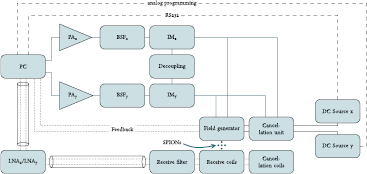
Figure 1. Signal chain of the MPS device. The signal is generated by a controlling computer (PC) and amplified by two power amplifiers (PA). The signal is then filtered by a band-stop filter (BSF). To achieve a good power transfer to the field generator, a capacitive impedance matching network is applied (IM). Additional DC paths are connected to the field generator which are programmed by the PC. The receive signal of the SPION's is recorded by receive coils, is filtered and then amplified by a custom low-noise amplifier (LNA). The coupling of the excitation signal is suppressed by a dedicated cancellation unit (Graeser et al 2013). The resulting signal is then digitized by the IO-cards.
Download figure:
Standard image High-resolution image2.1. Signal generation and acquisition
The system is controlled by a PC with a send and receive board by innovative integration (II). The transmit (Tx) signal is generated by the DAC channels of the X3-A4D4 (2009b) board. The resulting voltage across the transmit coils is used as a feedback signal for controlling the flux density inside the measurement chamber. The X3-A4D4 generates the signal with a sampling frequency of 4 megasamples per second (MSPS), assuring a high quality signal. The receive (Rx) signal is recorded by the X3-10M (2009a) receive board. The board has a maximum sampling frequency of 25 MSPS, which is limited to 17.5 MSPS to reduce data rates. Both cards are synchronized by the X3-timing module (X3-Timing 2009c) which provides a common clock and trigger to both cards.
2.2. AC power amplifiers
The generated signal has to be amplified in order to provide the necessary power for the field generator. As amplifiers add distortions to the signal, filter stages are needed to ensure a sufficient signal purity. To reduce demands on the filter stages, a high quality amplifier with low total harmonic distortion (THD) is chosen. For the presented system the class A/B nx200 amplifier module by Holton precision audio (http://holtonprecisionaudio.com/) is used. This module provides ultra low distortion and reduces the necessary effort on the filter stages.
2.3. Signal filtering
The amplifier provides high quality output signals. As the particle signal is usually several orders of magnitudes smaller than the direct feedthrough of the field generator, the remaining signals still cause a strong background signal. Therefore, the signal purity is enhanced by a passive Butterworth T-filter. The spectrometer is operated at different frequencies around 25 kHz to match the different trajectory field sequences of scanning devices (Buzug et al 2012, Goodwill et al 2012a, 2012b, 2013, Vogel et al 2014, Bente et al 2015, Panagiotopoulos et al 2015, Gräfe et al 2016). Therefore, the filter pass-band has to be sufficiently broad to include all the applied frequencies. The stop-band of the filter shall sufficiently damp the higher harmonics to reduce the direct feedthrough in the particle signal bandwidth. As the quality factor and therefore the filter performance scales with the volume of the inductors, the good amplifier performance allows for reducing the overall filter volume.
2.4. Field generator and receive coil setup
The field generator is the central part of the MPS. All coils have to provide a high homogeneous field profile, in order to avoid different excitation field values. A model and the implementation of the field generator and receiver is given in figure 2.
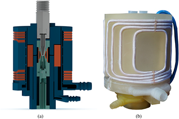
Figure 2. CAD model and implementation of the field generator. The presented setup is implemented twice for particle excitation and cancellation of the direct feedthrough.(a) CAD model. (b) Implementation.
Download figure:
Standard image High-resolution image2.4.1. Field generator.
For the x-channel, the homogeneity is achieved by using a solenoid coil with an inner diameter of 32.9 mm, an outer diameter of 50.95 mm, and a cylinder length of 30.2 mm. It consists of 36 turns realized with  μm litz wire resulting in an inductance of L = 36 μH with a measured resistance of 23 m
 at 25 kHz. The resulting field was simulated by a Biot–Savart approach and results in a maximum relative field error of
  within the measurement volume. The orthogonal Y-coil is designed as a rectangular saddle coil. The optimal current density distribution on a infinite cylinder for generating a homogeneous field is given by

with  being the current density distribution,
  being a unit vector on the z axis and φ and z being the cylinder coordinates (Lobb 0168, Sattel et al 2013). This continuous current distribution is approximated by discrete wire positions.
2.5. Send-receive decoupling
The send and receive path feature a mutual inductance causing a direct feedthrough of the excitation signal. As this signal is usually more than 4 orders of magnitude higher than the particle signal, one has to apply a signal separation strategy. While most imaging devices use a bandstop filter to separate the narrow band excitation signal from the broad band particle signal, other techniques as cancellation or perpendicular sensing are possible (Graeser et al 2013, Reeves and Weaver 2014). In the presented device the field generator is doubled as a cancellation unit, which is generating the exact same field topology (Graeser et al 2013). By changing the orientation of the cancellation coils the induced signal in the receive coils LcancRx have a  phase difference compared to the signal in the receive coils LRx. With a mechanical mechanism to adjust the coupling of the cancellation coils, an attenuation of 75 dB can be achieved. The limit of this attenuation is caused by parasitic elements of the inductors, which cause a phase shift error. However, the achieved damping is sufficient, as the remaining excitation signal can be subtracted by an air measurement. One drawback of this step is that the coil noise is doubled due to the identical construction of the coils. As the coil noise is still very low (
 m
m ) the system still provides a high signal to noise ratio (SNR).
2.6. Crosstalk decoupling
As the field generator consists of two coils sets for Bx and By field generation, an imperfect orientation of those coils causes crosstalk both in the send chain and the receive chain. Due to the impedance matching of the coils to the desired impedance of the amplifier, the crosstalk is amplified. The presented field generator has a measured coupling coefficient of k = 0.0095 which leads to a current ratio of  when sending only on the x-channel. To avoid this, a decoupling capacitor between the sending coils is introduced. With this capacitance the current ratio is reduced to Franke et al (2014)

The crosstalk of the receive channels to the orthogonal sending channel is addressed by adding low order filter stages that damp the signal to fit the dynamic range of the recording ADC.
2.7. Analog receive signal processing
In order to match the input voltage of the ADC, the signal is amplified by a custom built low–noise amplifier (LNA). It consists of a jFET input stage and two additional operational amplifier stages. The overall input noise of the amplifier is 440 pV/ with a gain of 55 dB (Biederer et al 2009). The system noise is dominated by the ADC noise and therefore a noise matching is only necessary for high diluted samples.
2.8. Offset field generation
A DC source is added to the electrical circuit to provide offset fields to the oscillating fields. A band-stop filter is set between source and the field generator to protect the DC sources from high AC currents. This filter is built up by using the cancellation unit in combination with a parallel capacitance, which results in a resonant band-stop. As the voltage over the coils stays nearly the same, the flux density in both coils is nearly identical. Therefore the cancellation unit can be used for two purposes, first to cancel out the direct feed through and second to reduce the oscillating current through the DC source. The DC sources are programmed by an analog signal from the IO-cards and a digital signal from the PC. With this setup it is possible to add any offset field amplitude in the range of ±21 mT.
2.9. Cooling
The mechanical mount of the field generator is produced by a 3D Systems ProJet HD 3200 rapid prototyping machine. This allows building up a very straight forward air cooling. Pressurized air is connected to a volume inside the field generator and follows predefined ways to the outside of the system. This way the maximum temperature of the coils is reduced.
2.10. Calibration
As the filter and amplification stages in both the transmit and receive chain transform the amplitude and phase of the signals, these signals have to be corrected to reconstruct the desired physical quantities. In this section, the measurement process to determine this transformation, called transfer function is given.
2.10.1. Receive chain calibration.
The voltage of the received signal can be described by the Faraday's law of induction and can be written as (Knopp and Buzug 2012)

Here,  is the receive chain sensitivity,
  is the permeability of free space,
  is the magnetization of the sample, t is the time and
  the spatial coordinate. From equation (2) it can be seen, that higher frequencies are amplified due to the derivative. This introduces a linear distortion in the frequency spectrum. In addition, other components of the receive chain are causing distortions to the amplitude and phase of the signal. To correct for those distortions, the transfer function describing the transformation from the magnetic moment to the measured voltage has to be recorded. This is done by a 3 mm circular calibration coil, wound with 100 μm copper wire with a total of 16 turns for the x-direction and 13 windings for the y-direction. The coil is connected to a 50
  series resistor, which allows measuring the current. Then a 5 kHz ramp signal is applied to the coil. This ramp signal contains of multiple harmonics of the fundamental frequency and therefore covers the whole bandwidth of the system. As the different trajectories result in various receive frequency components between the calibration grid points the missing grid points are interpolated in between. The resulting magnetic moment is then determined by

with N being the number of windings, A being the enclosed cross section, I being the applied current and  being the normal vector on the enclosed cross section. The transfer function of the system can be calculated by the Fourier coefficients of the applied magnetic moment and the received signal


The resulting transfer function can be seen in figure 3.

Figure 3. Transfer function of the setup measured for the x-channel and y-channel. The x-channel provides a nearly 3 times better SNR due to the higher coil sensitivity. However, the bandwidth of the y-channel is very high, which allows the application of a noise-matching afterwards (Zheng et al 2013).
Download figure:
Standard image High-resolution image2.10.2. Transmit chain calibration.
The transmit chain calibration is done by the same calibration coil used in section 2.10.1 and a voltage divider, which records the voltage of the transmit coil. To measure the field applied by the field generator, the voltage across the geometrically well known calibration coil  is recorded. With this voltage, the magnetic field can be reconstructed by Faraday's law of induction. The applied magnetic field is then given by

Recording the voltage divider signal at the same time as ucal, the amplitude ratio and phase of both signals can be calculated. Thereby, the correct field amplitude and phase can be assured by a software control circuit. As the impedance of the coil is frequency dependent, this has to be done for every applied frequency.
2.10.3. Offset field calibration.
The offset field is calibrated by measuring the offset field strength with a hall probe. By applying a defined current, the current to offset field ratio can be determined. This current is automatically controlled by the DC source.
2.11. Generation of the trajectory sequences
In order to generate different field sequences, an analytical description of the field is needed. Therefore, the field sequences of four possible measurements are presented below.
2.11.1. 1D sequence.
For the one dimensional sequence a fundamental frequency of  is chosen for perfect power matching. As the x-channel provides a better sensitivity due to the more sensitive coil geometry, it is chosen for one dimensional trajectory. The field sequence is then described by

The offset field can be added in both directions to be able to sense in the orthogonal direction.
2.11.2. Radial sequence.
The radial field sequence can be achieved by a modulation of the signals on both channels. Therefore a modulation frequency fm is introduced. The resulting field sequence is then given by

with  and
and  . As a result, the orientation of the field vector rotates within the measurement chamber with the frequency fm and changes its amplitude with the frequency f0.
2.11.3. Spiral sequence.
The spiral sequence is also modulated with a modulation frequency fm. The resulting field is given by

with  and
and  . The resulting field vector changes its orientation with the frequency f0 while the amplitude is modulated with the frequency fm.
2.11.4. Lissajous sequence.
The Lissajous sequence is generated by frequencies on the coils sharing a common base frequency. For the presented setup, the x-channel can send with a frequency of  or
or  . The y-channel sends with a frequency of
  This results in a repetition time of
  or
or  . The field equation results in

2.12. Particle samples
All the trajectories were applied to 10 μl undiluted Resovist (500 μ mol ml−1). This material consits of iron oxide nanoparticles which varies in shape and size. As Resovist is clinically approved for MRI studies it is often used as reference sample in MPI. A detailled analysis including particle parameters was performed in several studies (Eberbeck et al 2011, Yoshida et al 2013). In addition, the offset field is adapted for each particle position in an ideal gradient field. Hence, a full set of particle responses of an ideal imager is acquired. These measurements can be translated to a system matrix (SM) for an arbitrary MPI imager by applying the corresponding transfer function. Without loss of generality, an excitation strength of 14 mT, with offset fields between ±21 mT have been chosen.
3. Results
3.1. SNR
The SNR has been determined in frequency domain by comparing the spectral response of a 10 μl sample Resovist to the standard deviation of an empty measurement after subtraction of the background. The presented data was acquired with a Lissajous sequence with and a trajectory repetition time of  s resulting in a measurement time of 0.13 s averaging 200 times. The sensitivity of the setup was measured by a dilution series with Resovist to be at 450 pg Fe content. The SNR of the system is highest for the third harmonic and exceeds 105. In comparison to an imaging system the system provides a SNR improvement of roughly 100 to 1000. In figure 4 the background and signal spectra as well as the calculated SNR for the system is shown.
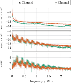
Figure 4. Standard deviation of the empty measurement (upper plot), signal intensity (middle plot) and SNR (lower plot) for the two receive channels. All measurements were taken at 14 mT with 200 averages and 1 repetition resulting in a measurement time of 136 ms. The x-channel has a better coil sensitivity and therefore a lower noise after transfer function correction. The setup is currently discretization noise dominated. As the sample chamber provides a homogeneous excitation for up to 100 μl particle solution, the SNR is defined by the dynamic range of the ADC.
Download figure:
Standard image High-resolution image3.2. 1D
As the SNR is very high the time domain signal can be used to determine the relaxation time constant of the particles to apply relaxation deconvolution in imaging (Bente et al 2015). Up to 80 harmonics can be detected in Fourier space depending on the particle sample and excitation strength. When acquiring the 1D particle response with offset fields in two directions, the resulting data set can be visualized as a 2D SM. Figure 5 shows this acquired SM. In general it can be stated that two samples can be separated in image reconstruction if there is a frequency component where the patterns show a sufficiently high difference either in amplitude or in phase. For a detailed analysis of SM's it is referred to the work of Rahmer et al (2010, 2009), Rahmer et al (2012). The acquisition time for the SM was 12 min for 10 averages. It can be seen that the signal causes a wide spreading in the y-direction which is referred to as haze. This effect has been extensively investigated with respect to the x-space approach. As the spectrometer is equipped with an orthogonal receive coil, the magnetization in y-direction can be displayed as well. The measured signal corresponts to a pMPI signal introduced by Reeves and Weaver (2014) and Weaver (2015). Figure 6 shows the real part of one selected system function. It can be seen that the signal phase and amplitude differs in the y-direction. This enables the reconstruction algorithm to reduce the blurring caused by the spreading of the system function in x-direction.

Figure 5. Absolute values of the system functions in case of line scan excitation. 10 μl Resovist have been excited by a field strength of 14 mT. As it can be seen the signal causes a haze in y-direction which has been investigated extensively in x-space. The measurement time for the SM acquisition was 12 min. (a) f = 52.371 kHz. (b) f = 230.115 kHz. (c) f = 458.643 kHz.
Download figure:
Standard image High-resolution image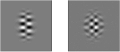
Figure 6. Real part (left) and imaginary part (right) of the system function component with f = 429.28 kHz. The induced voltage in the y-coil is zero for a particle sample in the center. For off center positions the amplitude rises and a show different phase encoding depending on the position. This phase information may enable the reconstruction process to reduce haze caused by the spreading of the signal in the x component.
Download figure:
Standard image High-resolution image3.3. Lissajous sequence
For more dimensional excitation the system function (the spatial dependency of one frequency component) is commonly used as a visualization of the receive signal. These spatial dependency is a measure for the achievable resolution by the particle sample (Rahmer et al 2009, Schmidt et al 2016). As the spectrometer resolves about 2.000 frequency components per channel they cannot entirely be shown here. Instead a small set of exemplary system functions is given. As it is common for multidimensional encoding sequences, the system function representation of three frequency components is shown in figure 7. The acquisition time for the SM was 12 min for 10 averages.

Figure 7. Absolute values of the system functions in case of Lissajous excitation with 14 mT of 10 μl Resovist for three selected frequency components. The measurement time for the SM acquisition was 12 min. (a) f = 52.371 kHz. (b) f = 223.767 kHz. (c) f = 458.643 kHz.
Download figure:
Standard image High-resolution image3.4. Spiral
The 2D spiral sequence is of interest for studying the particle dynamics. It is not suitable as an imaging trajectory, as it has a fading signal generation in the center of the image volume (Knopp et al 2009). In addition, the fast rotation of the field vector causes a dephasing of the particle easy axis leading to a broader and smaller particle response. A comparison of the particle signal with the signal of a Lissajous sequence is shown in figure 10. The measured SM of the spiral sequence is shown in figure 8. The acquisition time was 24 min for the  grid, which is caused by the longer trajectory repetition time (10 ms) compared to the Lissajous sequences.

Figure 8. Absolute values of the system functions in case of spiral excitation with 14 mT of 10 μl Resovist for three selected frequency components on a  grid. The measurement time for the SM acquisition was 24 min. (a) f = 50.3 kHz. (b) f = 77.2 kHz. (c) f = 384.8 kHz.
Download figure:
Standard image High-resolution image3.5. Radial sequence
Radial sequences are used in field free line (FFL) scanning devices (Weizenecker et al 2008, Knopp et al 2010, Erbe et al 2013). The FFL sequence has time varying offset fields which cannot be generated by this device. However, a radial sequence of an FFP can be generated by the MPS for particle analysis purposes. As for the spiral trajectory the repetition time is 10 ms leading to a acquisition time of 24 min. The resulting SM can be seen in figure 9.

Figure 9. Absolute values of the system matrix in case of radial excitation with 14 mT of 10 μl Resovist for three selected frequency components on a  grid. The measurement time for the SM acquisition was 24 min. (a) f = 50.3 kHz. (b) f = 77.2 kHz. (c) f = 384.8 kHz.
Download figure:
Standard image High-resolution image3.6. Signal comparison
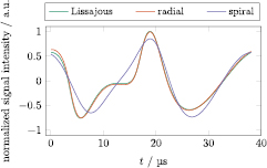
As it has been recently shown in simulation studies, the particle signal generation process is deeply connected to the field sequence that the particle experiences. Therefore, the signal of three different trajectories for the same particle sample are compared to each other. As the spiral trajectory has no signal induction in the center (Knopp et al 2009), an offset position was chosen. The signal has been corrected for the field derivative and normalized to the maximum signal intensity. The result is shown in figure 10.
Figure 10. Comparison of the particle signal generated by the Lissajous, radial and spiral trajectory at the FFP transit. As the velocity of the FFP is identical for all three trajectories at this time point, all signals are normalized to the overall maximum signal intensity. While the radial and Lissajous signal match each other nearly perfectly, the spiral signal shows a much broader slope. This would lead to a lower spatial resolution in imaging device. It verifies the results of simulations for the different trajectories (Graeser et al 2015b).
Download figure:
Standard image High-resolution image
The particle response of the Lissajous and radial sequence are nearly identical. However, the particles are unable to follow the fast field vector rotation of the spiral trajectory and therefore are not excited in their preferred direction. This results in a wider point spread function (PSF) which confirms the results of the simulation study in Graeser et al (2015b).
4. Conclusions
A two-dimensional MPS has been presented, which enhances the possibilities of the state of the art spectrometers by a various set of excitation schemes. It has been shown that the device is capable of applying four different types of excitation sequences while providing a very high SNR. It is able to calibrate arbitrary imaging devices as long as a good model of the field generator and receiver is given. The improvement in image quality is shown in a publication in this same journal issue (von Gladiss et al 0000). In addition, the signal acquisition is very fast allowing up to 200 measurements a second with various offset fields. However, the resulting SM's measured with the device rely on a good field model. For very inhomogeneous field profiles i.e. of a single sided device, the different field profiles of all transmitting coils have to be taken into account. If the magnet of the imager is therefore not homogeneous enough the field profile has to be measured in advance i.e. by a spherical harmonics approach to address this issue (Bringout and Buzug 2014).
The high signal quality allows analysing the particle signal in time space without postprocessing as frequency selection or additional filtering. The results show a dependency between the PSF and the field sequence. As the PSF is a direct measure for the spatial resolution, fast rotations in the trajectory should be avoided (Goodwill and Conolly 2010).
Due to its high SNR and its flexibility of driving different trajectories, the presented device is very useful in order to investigate the behavior of magnetic nanoparticles. As the generation of the particle signal is still not fully understood, the device provides data which allows for understanding the particle physics for multidimensional imaging.
Acknowledgments
We thankfully acknowledge the financial support of the German Research Foundation (DFG) and the Federal Ministry of Education and Research (BMBF) (Grant Numbers BU 1436/10-1 and 13GW0069A).