


Abstract
To effectively monitor the operation state of in-wheel motors used in electric vehicles and ensure the safety of the whole vehicle, a diagnosis method based on hidden Markov model (HMM) and Weibull mixture model (WMM) is proposed for mechanical faults in in-wheel motors, known simply as the WMM-HMM diagnosis method. Firstly, vibration signals of the in-wheel motor are extracted for sensitive symptom parameters which are used to characterize the operation state and establish the observation sequence. Secondly, WMM is employed to expand the limited observation sequence under various operating states of in-wheel motors to obtain sufficient observation sequence as the training sample set of HMM, and HMM parameters are determined through combining supervised learning with unsupervised learning algorithm. Then the WMM-HMM diagnosis models are constructed under low and medium speed conditions respectively. Finally, the corresponding faults in-wheel motors are customized and the test bench is built to verify the proposed method. The test results show that the proposed method can accurately identify the mechanical fault state of in-wheel motors under different conditions and has good generalization and applicability in traditional methods comparison.
Export citation and abstract BibTeX RIS
1. Introduction
Due to the problems of resource consumption and environmental pollution brought by traditional fuel vehicles, research and manufacturing of environmental-friendly new energy vehicles have developed rapidly [1, 2]. Electric vehicles driven by in-wheel motors have unique advantages such as compact structure and flexible control, and have become a research hotspot in the development of the new energy vehicle industry [3, 4]. However, since the in-wheel motor is installed in the wheel hub directly, not only will it inevitably bear the pressure from suspension and road impact, but also easily wear parts in the process of operation, leading to mechanical faults. Moreover, in-wheel motors integrate multiple important functions such as driving, braking and loading, so play an important role in the wheel drive system of electric vehicles. Once a certain mechanical fault of in-wheel motor occurs, the operation safety of the whole vehicle will be influenced, and even the driver and passenger will be endangered [5, 6]. Concerning the issues mentioned above, it is crucial to detect and diagnose the faults that may occur during the operation of in-wheel motors.
In recent years, most intelligent classification algorithms have been widely used in the field of fault diagnosis such as support vector machines [7], artificial neural networks (ANNs) [8], convolutional neural networks (CNNs) [9], artificial hydrocarbon network [10], generalized linear regression model [11] and deep belief network [12, 13]. These have certain guiding significance for diagnosing mechanical faults of in-wheel motors. However, traditional fault diagnosis and monitoring methods usually use the single-stage information of operation state to infer whether there are faults or not, and lack comprehensive judgment on the basis of the multi-stage information, especially incipient faults or intermittent faults. Hence, multi-stage information processing algorithms are combined gradually multiple features related to target types at different moments to overcome the limitations of relying on single-stage information. Hidden Markov model (HMM) [14] and dynamic Bayesian networks (BNs) [15] are representative examples that are applied in the field of fault diagnosis.
As a kind of time-series probability model, HMM can estimate the change of hidden state chain by the recurrence of time series. In view of the effective and mature intelligent classification capabilities, numerous works based on HMMs have been reported in fault diagnosis [16–18] and it can be combined with other intelligent algorithms to improve diagnosis efficiency. For example, Wang and Du [19] used the sparse dictionary self-learning method to extract bearing features and built HMM based on this, which improved the recognition accuracy of rolling bearing composite faults. Li et al [20] proposed a combination of spectral kurtosis based on Choi-Williams distributed HMM, used the local mean decomposition algorithm to decompose multi-component signals and extracted fault features as the HMM's input, effectively identified the initial fault characteristics of the gearbox. Don and Khan [21] trained an HMM with standard operating condition data while the structure of BN was developed based on process knowledge, and used the updated BN for fault diagnosis by considering the corresponding changes in probability. These studies illustrate the potential of HMM in the field of fault diagnosis, and prove that a large amount of data is required in the process of constructing HMM to train and optimize the parameters for obtaining the best diagnosis results. However, electric vehicles driven by in-wheel motors have diverse driving conditions and complex operating environments, then it is not only difficult but also expensive to collect a large amount of observation data in the actual driving process. This will cause the diagnosis results of HMM to fail to achieve high diagnostic accuracy when using small sample observation data for fault diagnosis.
An effective method is to acquire a small amount of data and expand the original data according to a certain data fitting method to obtain more training data. Therefore, choosing a suitable data fitting model is of great significance to the subsequent diagnosis results. The common method of combining data fitting with HMM is Gaussian mixture model (GMM) [17], which is commonly used in the field of speech recognition [22–25]. The observation probability matrix in the HMM parameters can be described by the GMM of the observation sequence, and the corresponding recognition model can be obtained. Yao et al [26] used GMM to depict two-dimensional observation probability density of each state, and constructs the HMM model by considering the state changes of traffic during the communication. Yuan et al [27] illustrated the problem of stability induced by k-means clustering and applied GMM to the unified initialization of guided wave-HMM, and verified in damage evaluation experiment. Aiming at the problem that part of the discretization range was not achievable in the observation state calculation process, Zhang et al [28] used multi-dimensional GMM to fit motion data to build a GMM-HMM recognition model, which can obtain accurate hidden state numbers according to key frames. The above studies are all based on the premise that the observational data conforms to the Gaussian distribution. However, during the actual operation of the in-wheel motor, some signals do not completely conform to GMM. Therefore, using GMM to perform data fitting on these signals often fails to obtain ideal diagnosis results.
For most mechanical and electrical products, the distribution of wear cumulative failure conforms to Weibull distribution, and based on which Weibull distribution is widely used in reliability engineering and related data fitting. Chu et al [29] used the deep survival model of discrete Weibull distribution to learn potential features, an integrated deep learning method with CNN and long-short-term memory network was proposed to realize the capture of the failure degradation trend of turbofan engine and the estimation of service life. Gao and Yuan [30] utilized the Weibull distribution and reliability analysis theory to obtain the basic assumptions of fatigue life and fatigue damage, a probability model of fatigue damage accumulation was proposed. It was verified that the proposed model can quantify the dynamic probability characteristics of fatigue damage accumulation. According to the above related research, a single Weibull distribution is widely used in the field of reliability testing and fault diagnosis.
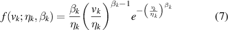
Therefore, in view of the great data fitting performance of Weibull distribution, a mechanical fault diagnosis method for in-wheel motors based on the basic HMM and Weibull mixture model (WMM), referred to as WMM-HMM diagnosis method is proposed in this paper. As shown in figure 1, highly sensitive symptom parameters (SPs) are extracted from a small amount of observation data, and Weibull distribution fitting is performed to achieve data expansion. Sufficient data constitutes a training sample set to train and update and optimize HMM's parameters, thereby constructing WMM-HMM, and using the model to monitor and diagnose the fault status of in-wheel motors in real-time. The arrangement of this paper is as follows: section 2 focuses on the construction of WMM-HMM, and expounds involved Weibull distribution, WMM and HMM. In section 3, the effectiveness of the proposed method is verified by a specific in-wheel motor bench test. The conclusion and prospect are given in section 4.
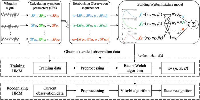
Figure 1. WMM-HMM's construction and application.
Download figure:
Standard image High-resolution image2. Hidden Markov model based on Weibull mixture model (WMM)
2.1. Hidden Markov model
HMM is a statistical model and uses a Markov process that contains hidden and unknown parameters for predicting functions of uncharacterized sequences [31]. In the model, the observed parameters in each state are used firstly to generate an observation random sequence for identifying the hidden parameters, and secondly, hidden Markov chains can be formed to generate an unobservable state random sequence, and finally, the further analysis will be performed. Here, a Markov chain is a discrete-time process for which the next state is conditionally independent of the past given the current state. Each state has a discrete or continuous probability distribution over possible emissions or outputs. When one state transitions to another state or a specific state is visited, the output will be generated. What guides the state-to-state transition is a set of transition and emission probabilities. The transition probability is the probability of moving from one state to another via a connected edge, and the emission probability is the probability of emitting a especial symbol at a state. The probability of any sequence is computed by multiplying the emission and transition probabilities along the path.
Formally, a complete HMM has a combination of three basic parameters λ = ( π, A, B ). The parameters π and A are used to describe the Markov chain and the stochastic process is described by parameter B [32]. Here π is the probability distribution of operating state in initial time t 0, it defines the probability distribution in hidden state π = [π1, π2, ..., πi , ..., πN ]. A is the state transition matrix, where A = [aij ]N ×N , the element aij in the matrix reflects the probability from one state Si (t) at time t to another state Sj (t+ 1) at time t+ 1. B is the observation probability matrix, where B = [bjm ]N ×M , and its element bjm represents the probability of obtaining the observed value in state Sj . The specific elements in the matrix are described as follows:


where Si denotes the ith hidden state and qt denotes the hidden state at time t, P(·) expresses the probability value. Let N be the number of possible hidden states, then the states set is described by S = [S1, S2, ..., Si , ..., SN ], and qt ∈ S. v (m) is the mth observation output and O t is the observation output at time t. Let M be the number of all possible observation outputs, then the observation matrix is described by V = [ v (1), v (2), ..., v (m), ..., v (M)], and O t ∈ V .
In practical engineering applications, a time-slice is regarded as an observation phase, then the observation outputs from multiple successive time-slices can be formed an observation sequence O = [O1, O2, ..., Ot , ..., OT ]. Similarly, the corresponding hidden state sequence Q = [q1, q2, ..., qt , ..., qT ] is labeled. Based on the prior data or expert experience, the initial parameter set λ 0 = ( π 0, A 0, B 0) is usually obtained [33]. In the follow-up process, there are two essential problems. One is the model parameter estimation that is to determine the most likely values of HMM's parameters according to the observed series of history training data. Another is the condition recognition that to find the most likely hidden value sequences.
For updating new basic parameters
λ
= (
π, A, B
) of HMM, when there are a lot of prior data that the observation outputs and the corresponding hidden states are known, Baum–Welch algorithm is usually used to train the parameters
λ
of HMM in actual application [34]. Given an observation sequence
O
, Baum–Welch algorithm can find a local maximum
λ
= (
π, A, B
) =  for observation sequence
O
with random initial conditions, where
for observation sequence
O
with random initial conditions, where  is the estimated value of
λ
at present. The algorithm can be described as follows:
is the estimated value of
λ
at present. The algorithm can be described as follows:
When the error threshold or maximum number of iterations is satisfied, the optimal parameters are obtained and marked as λ * = ( π *, A *, B *), then the most basic HMM has constructed. At the condition recognition stage, Viterbi algorithm is used to decide the most probably hidden state sequence on the basis of a new observation sequence [35].
In general, GMM is used to fit the characteristics of the observation data in the process of HMM's construction. However, there are some observation data that disobey a random Gaussian distribution in the real, and then it will highlight approaches and solutions on how to effectively fit the especial observation data.
2.2. Weibull mixture model
Weibull distribution is a two-parameter or three-parameter family of curves, which gives an approximate but generally good fit to some especial observation data, especially in reliability and lifetime modeling. Certainly, two-parameter Weibull distribution is a special case of the generalized three-parameter gamma distribution. Compared with Gaussian distribution and exponential distribution, Weibull distribution is more flexible, versatile and relative simplicity, and then is widely used in reliability engineering and predictive data analysis. In the field of condition monitoring, Weibull distribution is often selected to describe the variation trend of any one SP extracted from vibration signals [36]. When many SPs are used to evaluate an analytic target, WMM is performed to exploit their talent.
Let K be the number of observation parameters in HMM mentioned above, each observation output can be denoted as v (m) = [v1(m), v2(m), ..., vk (m), ..., vK (m)]'. Then the same observation parameter gathers in each row of observation matrix V . For analyzing the same observation parameter, vk is used to express the kth observation parameter in observation matrix, then v k = [vk (1), vk (2), ..., vk (m), ..., vk (M)] and V = [ v 1, v 2, ..., vk,..., vK ]'. Suppose all observation parameters obey some kinds of Weibull distribution, the Weibull probability density function of v k may be expressed as follows:
where ηk > 0, βk > 0 are the scale and shape parameters, respectively. Accordingly, the distribution of the observation sequence V which is composed of K observation parameters can be described by WHH as follows:
where η and β are the sets of the scale and shape parameters. w = {w1, w2, ..., wK } is the set of weight coefficients. wk is the weight coefficient of the kth Weibull distribution, and satisfies the following conditions:
2.3. HMM based on WMM
In general, traditional HMM needs the global observation sequences. However, a fault condition of in-wheel motors is implicit in the real, especially in the earlier fault period, then it is difficult to observe directly the fault states of in-wheel motors. Usually, the condition signal such as vibration, noise or electric signal is collected to detect the anomalous change in the time, frequency or time-frequency domain, then extract the different SPs for reflecting the fault states of in-wheel motors [37, 38]. In that way, SPs in the running process of in-wheel motors can form many observation sequences, and observation sequences in the normal condition are more, but observation sequences in the fault states or transition process from normal state to fault states are lesser even no, especially in construction phase of condition monitoring system. When the limited observation sequences are used to establish a HMM of fault diagnosis, the parameter λ = ( π, A, B ) may be affected. Even an unsupervised learning algorithm such as Baum–Welch algorithm is not limited by the lack of training samples, it is sensitive to select the initial parameters λ 0 = ( π 0, A 0, B 0) [19]. When expert experience or random assignment is relied on, the iterative accuracy may be reduced to cause the insufficient parameters of HMM, and then reduce the diagnosis accuracy. In practical scientific research, there are different fitting methods applied in many fields to fit the experimental data, predict the global distribution, and obtain the global data. For example, a simple ANN is used to estimate the thickness, roughness and density of organic semiconductor thin films for obtaining various types of global data [39]. The backpropagation neural network is used to fit the true distribution of the original sample data, and the CNN is combined to improve the diagnosis accuracy [40]. Moreover, many SPs extracted from vibration and noise signals of in-wheel motor are selected to obey some kinds of Weibull distribution in the previous research [41]. Therefore, WMM is used to expand the limited data for obtaining the optimal parameters of HMM. The proposed method in the paper is known as WMM-HMM.
The approach of WMM-HMM involves three major steps. First, the limited observation sequences are used to confirm the parameters of WMM. Second, the optimal WMM is applied to obtain the global observation sequences. Third, the global observation data are utilized to optimize the parameters of HMM, and then build a diagnosis system of HMM, as follows:
Step 1: Solving the parameters η, β and w of WMM. It can be seen from the above description that the observation sequence V = [ v 1, v 2, ..., vk,..., vK ]' is composed of K SPs, and they are independent of each other. For the kth SP, the existing observation sequence v k can be expressed by [SPk (1), SPk (2), ..., SPk (m), ..., SPk (M)]. Then the two parameters ηk and βk of Weibull distribution can be obtained using the sample mean μk and sample variance σk 2 of the kth SP's observation value, the value of βk is estimated as the solution of:
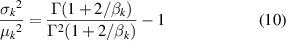
and the value ηk of is given by:
where Γ(·) is gamma function. In this way, the Weibull distribution of each SP can be determined.
For the weight coefficient set w in WMM, the state differentiation of SPs is analyzed to propose an objective weighting method. It is the basic idea of the method that Euclidean distances in a unit range between single SP and all SPs are accumulated to determine the SP's contribution, then the weight coefficient wk of the kth Weibull distribution can be expressed as follows.
where p(·) is the probability density function of Weibull distribution, Ed(·) is Euclidean distance. R is the number of the observation outputs in a unit range of the mth observation output. Certainly, the greater the difference, the greater the value of wk . With the determination of w , WMM of observation matrix is determined.
Step 2: Establishing the training sample set of HMM. Based on the determined WMM of observation matrix V , it is easy to build the fuzzy function of the corresponding hidden state sequence Q , which is denoted as Q = f( V ). Then the method of cubic convolution interpolation is used to extend the training sample set of HMM.
where F(·) is the hidden state function of the corresponding coordinate after interpolation. d k and Δ v k are the deviation value and sampling interval of v k , respectively. When the observation output is composed of multiple SPs, the corresponding hidden state is expressed by positive integer, round-function is used to ratiocinate the hidden state. In this way, the limited observation matrix V and the corresponding hidden state sequence Q can be replenished to obtain the global observation data, then establish the training sample set of HMM. In general, the training sample set is shown as [(Si 1, n1· v )1, (Si 2, n2· v )2, ..., (Sit, nt · v )t , ..., (SiT, nT · v )T ], where Sit and nt are the hidden states and the number of observation output at the tth time segment, respectively.
Step 3: Optimizing the parameters
λ
= (
π, A, B
) of HMM. With the increase of observation time, WMM is more realistic, the training sample set of HMM is more intact. For the initial parameters
λ
0 = (
π
0,
A
0,
B
0) of HMM, the statistical method such as count-function is used to determine tentatively. Let C1(Si
) be the frequency of Si
in initial time segment, C2(Si, Sj
) is the frequency of transferring from state Si
to Sj
in training sample set, C3(nm
·
v
) is the frequency of nm
·
v
obtained in state Sj
, the probability of each state πi
in the initial state vector
π
0 is calculated by  , each transition probability aij
from state Si
to Sj
in the initial transition matrix
A
0 is computed by
, each transition probability aij
from state Si
to Sj
in the initial transition matrix
A
0 is computed by  , each observation probability bjm
of state Sj
in the initial observation probability matrix
B
0 is counted by
, each observation probability bjm
of state Sj
in the initial observation probability matrix
B
0 is counted by  Once the initial parameters
λ
0 = (
π
0,
A
0,
B
0) of HMM are determined, Baum–Welch algorithm as shown in (4)–(6) is performed to obtain the optimal parameters
λ
= (
π, A, B
), then construct a WMM-HMM diagnosis model.
Once the initial parameters
λ
0 = (
π
0,
A
0,
B
0) of HMM are determined, Baum–Welch algorithm as shown in (4)–(6) is performed to obtain the optimal parameters
λ
= (
π, A, B
), then construct a WMM-HMM diagnosis model.
When a new observation sequence O test = [ O 1, O 2, ..., O T ] is known, the corresponding hidden state sequence can be concluded as follows:

In the paper, the running state of in-wheel motor is hidden, but vibration signal can be measured easily. Based on WMM-HMM diagnosis method, multiple SPs are extracted from vibration signal to build the observation sequence O , then the maximum likelihood state sequence S * of in-wheel motor can be inferred. When a fault of in-wheel motor occurs, it is easy to judge the fault condition and identify the fault type. The application of WMM-HMM method in in-wheel motor fault diagnosis will be described in the third chapter.
3. Experiment verification
3.1. Test bench of in-wheel motor
Figure 2 is the test bench of an in-wheel motor that contains three major sections, that is, electric wheel, road excitation and suspension system. The electric wheel is composed of a wheel and an in-wheel motor (Type: QSWP30030X; Rated power: 3 kW), which is controlled by STM32 single chip microcomputer for simulating the voltage of accelerator pedal. Road excitation is simulated by hydraulic exciter (Type: INSTRON 8800) that the excitation frequency and amplitude can be set on the basis of different road levels. Suspension system is composed of spring component, guides component and dampers, the top is fixed in table frame, a pressure sensor (Type: HD-YB-11LY; Sensitivity: 2.0 ± 0.005 mV V−1) is installed between the suspension bottom and the axle of the electric wheel. When the axle of the electric wheel is lifted to a certain height by the hydraulic exciter, the different loads can be simulated. Moreover, an accelerometer (Type: PCB333B30; Sensitivity: 100 mV g−1) is installed at the axle of in-wheel motor, vibration signals are collected with a 12.8 kHz sampling frequency at a relatively steady speed of 100, 200, 300...700 rpm. The sampling time is 90 s.
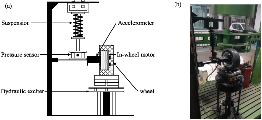
Figure 2. Test bench of in-wheel motor. (a) Flow diagram and (b) physical photo.
Download figure:
Standard image High-resolution imageIn order to research the operation states of in-wheel motors with mechanical faults, common bearing faults such as outer race fault, inner race fault, rolling element fault (Width: 0.3 mm; Depth: 0.1 mm) were artificially made to build on the stator axis of each in-wheel motor by professionals, respectively. In the experiment, in-wheel motors with mechanical faults are orderly exchanged to run with the other condition fixed.
3.2. Construction of diagnosis model
In order to verify the generalization and applicability of the proposed method, and weaken the influence of different speeds for the diagnosis model, the general standard of a vehicle low-speed, medium-speed and high-speed is used, and the radius of the electric vehicle is considered, the 100, 200, 300, 400 rpm speeds of in-wheel motor are collectively defined as low-speed condition; the 500, 600, 700 rpm speeds are regarded as medium-speed condition. Since the dynamic vibration and output torque of in-wheel motor are more differences under low-speed and medium-speed conditions, two types of fault diagnosis models are constructed, respectively. In practical application, the average value of operating speed during a monitoring period is used to judge whether in-wheel motor is operating in low-speed or medium-speed condition, then the corresponding diagnosis model is selected.
Moreover, the operation state of in-wheel motors is a gradual degradation process during its evolution, that is, in-wheel motor can only transfer from normal state to fault state, but not transfer from the fault state to the normal state, and not transfer from one fault state to another fault state. Certainly, a single fault may evolve into a compound fault. Therefore, the hidden state of in-wheel motors is a non-cross-type Markov chain as shown in figure 3. For example, outer race fault of a bearing can easily lead to rolling element defect, and then form a compound-fault state that includes outer race fault and rolling element fault at the same time [42]. As time goes on, inner race is involved in fault state.
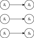
Figure 3. Non-cross-type Markov chain.
Download figure:
Standard image High-resolution imageIn the paper, single fault state of in-wheel motors is focused, and a sequential diagnosis system is designed for improving the accuracy of fault identification. Firstly, inner race fault is regarded as the primary task of detection. In the following steps, outer race fault and rolling element fault are diagnosed one by one. Then WMM-HMM diagnosis models from normal state (S1) to inner race fault (S2), outer race fault (S3) or rolling element fault (S4) are constructed for in-wheel motor, respectively. Certainly, the diagnosis goal is different in each step, the input parameters of each model may vary. Here, the WMM-HMM diagnosis model from S1 to S2 under low-speed condition is regarded as an example, the construction process is introduced in detail.
3.2.1. Symptom parameters (SPs).
In general, the sensitivity of each SP is different under different conditions, it is not easy to find effective SPs for some faults [43]. Moreover, too few SPs cannot distinguish multiple fault types at the same system [10], but more SPs must come to being data redundance, data exchange difficulty and work inefficiency [37]. Therefore, there are some methods such as distinguish index (DI) [44] and stable average discrimination rate (SADR) [38] that have been used to select moderate and high-sensitive SPs for fault diagnosis and identification. Here, two methods of DI and SADR are combined to select three SPs for three mechanical faults of in-wheel motors, respectively. As far as the WMM-HMM diagnosis model from S1 to S2 under low-speed condition, three SPs such as root mean square, skewness and waveform deviation rate are decided, as follows:
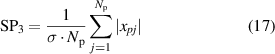
where {xi
} (i = 1–N) is the sequence of vibration signal,  and σ are the average value and standard deviation of {xi
}. {xpj
} (j= 1–Np) is the peak value of {xi
}, Np is the total number of {xpj
}.
and σ are the average value and standard deviation of {xi
}. {xpj
} (j= 1–Np) is the peak value of {xi
}, Np is the total number of {xpj
}.
When 2 s are regarded as an observation period, the corresponding SP1, SP2 and SP3 are calculated according to the vibration signals of in-wheel motor, and then the SP sequences of SP1, SP2 and SP3 are obtained with 45 observation time periods. Each SP sequence is analyzed, the statistical results are fitted with Gaussian distribution and Weibull distribution, respectively, as shown in figure 4. It is obvious that each SP is more in line with Weibull distribution than Gaussian distribution. Certainly, the method of statistical test can be used to prove that these SPs conform to Weibull distribution.
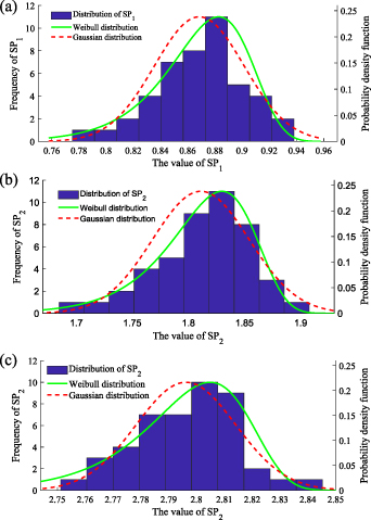
Figure 4. Statistics of SPs and corresponding probability density functions: (a) SP1, (b) SP2 and (c) SP3.
Download figure:
Standard image High-resolution image3.2.2. WMM construction.
For normal state (S1) and inner race fault state (S2) of in-wheel motors under low-speed condition, the limited observation sequences with the known state sequences are organized into the training data, respectively. Formulas (10)–(12) are used to calculate two parameters ηk, βk and the corresponding weight coefficient wk of each SP in each state, as shown in table 1, then the WMM is constructed.
Table 1. WMM parameters.
| SP | η | β | w | |||
|---|---|---|---|---|---|---|
| S1 | S2 | S1 | S2 | S1 | S2 | |
| SP1 | 1.0031 | 1.0041 | 934.0 | 1151.3 | 0.3137 | 0.3244 |
| SP2 | 1.0029 | 1.0037 | 1084.5 | 1230.2 | 0.3600 | 0.3574 |
| SP3 | 1.0006 | 1.0008 | 1029.2 | 937.2 | 0.3263 | 0.3182 |
3.2.3. HMM establishment.
With the construction of WMM, the Weibull probability density function f (SP1, SP2, SP3) is known. Based on the original observation sequences, significance level of 0.01 is set to confirm the confidence interval of each SP, the deviation value d k and sampling interval Δ v k , formula (13) is used to extend the original observation data. Then new observation data under each condition is up to four times. Since there are 45 observation time periods of each state under each speed, new observation data are enlarged to 180, respectively. Therefore, half of the data is used to build the training samples.
Here, the training samples of HMM S1 to S2 under low-speed condition are regarded as an example to describe the composition and sample capacity. Since low-speed condition includes four kinds of speed, the training sample set is shown as [(S1, 90· v )T speed=100, (S1, 90· v )T speed=200, (S1, 90· v )T speed=300, (S1, 90· v )T speed=400, (S2, 90· v )T speed=100, (S2, 90· v )T speed=200, (S2, 90· v )T speed=300, (S2, 90· v )T speed=400]. Where v = [SP1, SP2, SP3], (·) T speed=S is the training sample at the time segment when the speed of in-wheel motor is S (S= 100, 200, 300, 400). Next comes the training parameters of HMM. When the supervised learning method mentioned in section 2 is used to obtain the parameters of HMM from S1 to S2 under low-speed condition are shown as follows:
Thus, the WMM-HMM diagnosis model from normal state (S1) to inner race fault (S2) under low-speed condition is established. Similarly, vibration signals of in-wheel motors with inner race fault under medium-speed condition are analyzed to select three high-sensitive SPs for observing the operating state, the original observation sequences are processed by WMM method to input the HMM, then it is easy to build the WMM-HMM diagnosis model from S1 to S2 under medium-speed condition. With the threshold judgment of operating speed, one of the two models will be performed to detect whether in-wheel motor is in inner race fault state. If the probability that the current state has been verified as inner race fault (S2) is high, the diagnosis system automatically stops. Otherwise, the system will come into the next step for the identification of outer race fault (S3) and rolling element fault (S4). In the same way, the operating state of in-wheel motor are diagnosed sequentially.
3.3. Diagnosis results
In order to verify the effectiveness of the WMM-HMM diagnosis system for mechanical faults of in-wheel motors, the remaining new observation data that includes normal state and three faults under low-speed and medium-speed conditions is taken as the test sample to test the recognition rate of each operating state of the in-wheel motor. The recognition rates of normal state (S1), inner race fault (S2), outer race fault (S3) and rolling element fault (S4) are shown in figure 5.
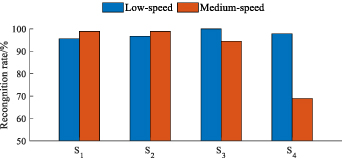
Figure 5. Experiment results in diagnosis system.
Download figure:
Standard image High-resolution imageObviously, each operating state has been recognized precisely, and the majority of recognition rates are more than 93.8%. There is only one case exception that 72.2% test cases of rolling element fault under medium-speed condition are diagnosed correctly. The reason is that the single filter with the fixed constraint is used to process the more overlap between the natural frequency of test bench and the characteristic frequency of rolling element fault under medium-speed condition. Overall, the WMM-HMM diagnosis system is available for diagnosing mechanical faults of in-wheel motor.
3.4. Comparison and discussion
To verify the effectiveness and applicability of the proposed method in the field of mechanical fault diagnosis of in-wheel motor, the following different comparative strategies are designed for analysis and discussion.
3.4.1. Comparison of the proposed method with different inputs.
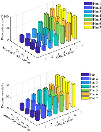
For the WMM-HMM diagnosis model from normal state (S1) to inner race fault (S2) under low-speed condition, seven different observation parameters as shown in table 2 are planned as the inputs of the diagnosis model to verify the importance of the observation sequence. Among them, plan 1, plan 2 and plan 3 use a single SP to build the observation sequence, plan 4, plan 5 and plan 6 use two SPs, plan 7 uses three SPs that is the proposed method in section 3.2. When the different SPs in each plan are input into the WMM-HMM diagnosis model, the recognition rate of each operating state is obtained as shown in figure 6.
Figure 6. Comparison of diagnostic results of different input schemes under different operating conditions: (a) low-speed and (b) medium-speed.
Download figure:
Standard image High-resolution image
Table 2. Different plans with the inputs of different SPs.
| Plan number | Input SPs |
|---|---|
| Plan 1 | SP1 |
| Plan 2 | SP2 |
| Plan 3 | SP3 |
| Plan 4 | SP1 and SP2 |
| Plan 5 | SP1 and SP3 |
| Plan 6 | SP2 and SP3 |
| Plan 7 | SP1, SP2 and SP3 |
It is apparent that the recognition rates in plan 1, plan 2 and plan 3 are generally low (less than 70%), the experiment results in plan 4, plan 5 and plan 6 have shown some improvement, but wave up and down, and the diagnosis accuracy in plan 7 is high and stable. Therefore, one or two SPs cannot effectively observe the operating state of in-wheel motor, even if they are high-sensitive. The reasons is that too few observation parameters cannot reflect a comprehensive features of in-wheel motor. In the paper, it is beneficial that three SPs are selected to represent the operating characteristic of in-wheel motor.
3.4.2. Comparison of different diagnosis methods.
Traditional HMM and GMM-HMM are often employed to detect fault and identify fault types [45]. Then the same experimental data above are used to establish the HMM and GMM-HMM diagnosis systems, respectively, and the same observation data are preprocessed as the testing data to verify the classification performance. The diagnosis results of different diagnosis methods are shown in table 3. Obviously, the train accuracies of three methods are close to 100%, but there is remarkable gap among the test accuracies. As a whole, the effectiveness of traditional HMM method is weakest, the average recognition accuracy is 59.72% only, it cannot meet the demands of practical engineering. The better one is GMM-HMM diagnosis method, the average diagnosis accuracy is improved by 81.11%, but the variability is greater. Certainly, the best one is WMM-HMM method proposed in the paper, the test results of each state in different speeds are more than 94%, and the average value ascends to 97.64%. It shows that WMM-HMM has advantages in the field of fault recognition.
Table 3. Diagnosis results of different diagnosis methods.
| Method | Running condition | State | Train | Test | ||
|---|---|---|---|---|---|---|
| Accuracy (%) | Time (s) | Accuracy (%) | Time (s) | |||
| WMM-HMM | Low-speed | S1 | 100 | 0.101 | 95.56 | 0.040 |
| S2 | 100 | 0.102 | 96.67 | 0.037 | ||
| S3 | 100 | 0.104 | 98.89 | 0.033 | ||
| S4 | 100 | 0.104 | 97.78 | 0.039 | ||
| Medium-speed | S1 | 100 | 0.095 | 98.89 | 0.035 | |
| S2 | 100 | 0.095 | 98.89 | 0.038 | ||
| S3 | 100 | 0.093 | 94.44 | 0.039 | ||
| S4 | 100 | 0.096 | 100 | 0.040 | ||
| Average value | 100 | 0.0988 | 97.64 | 0.0376 | ||
| GMM-HMM | Low-speed | S1 | 93.33 | 0.117 | 90 | 0.041 |
| S2 | 90.00 | 0.120 | 86.67 | 0.039 | ||
| S3 | 100 | 0.119 | 86.67 | 0.038 | ||
| S4 | 100 | 0.116 | 61.11 | 0.041 | ||
| Medium-speed | S1 | 100 | 0.102 | 90 | 0.040 | |
| S2 | 100 | 0.104 | 86.67 | 0.040 | ||
| S3 | 100 | 0.103 | 86.67 | 0.041 | ||
| S4 | 100 | 0.101 | 61.11 | 0.038 | ||
| Average value | 97.92 | 0.1103 | 81.11 | 0.0398 | ||
| HMM | Low-speed | S1 | 98.89 | 0.118 | 53.33 | 0.040 |
| S2 | 100 | 0.119 | 62.22 | 0.038 | ||
| S3 | 100 | 0.118 | 62.22 | 0.037 | ||
| S4 | 100 | 0.119 | 65.56 | 0.038 | ||
| Medium-speed | S1 | 100 | 0.087 | 68.89 | 0.036 | |
| S2 | 100 | 0.089 | 58.89 | 0.037 | ||
| S3 | 100 | 0.090 | 65.56 | 0.039 | ||
| S4 | 100 | 0.085 | 41.11 | 0.035 | ||
| Average value | 99.86 | 0.1031 | 59.72 | 0.0375 | ||
For examining the response rates of three algorithms above mentioned, the computer (Processor: AMD Ryzen 7 5800H; OS: Windows 11; Memory: 16G) is used to execute the training program and test application, then the running time of each method is also displayed in table 3. The average running times of WMM-HMM method in the training program and test application are 0.0988, 0.0376 s, the average times of GMM-HMM in two processes are 0.1103, 0.0398 s, and the average times of traditional HMM are 0.1031, 0.0375 s. Overall, the response speeds of three algorithms are faster, and there is little difference.
4. Conclusion
To effectively identify mechanical faults of in-wheel motors and judge the operating state in real conditions, WMM and HMM are combined to propose the WMM-HMM diagnosis method in this paper, and its superiority is summarized by the following points:
- (a)WMM can describe more precisely the SPs' variety of the operating state of in-wheel motor, then expand effectively to more observation sequences from the limited data. It is in fact the solution to the universal problem of fault diagnosis in actual engineering.
- (b)HMM can be used to detect a fault and identify the type, especially WMM is combined to build the diagnosis model, which not only avoids the randomness and uncertainty of traditional HMM's parameters in unsupervised learning algorithm, but also optimizes quickly the parameters of diagnosis model. It is attributed primarily to the capability of WMM and HMM.
- (c)WMM-HMM diagnosis system not only considers the effect on the observation information of speed alteration, but also pay attention to the difference of fault characters in different operating states. It shows the flexible adaptability of a sequential diagnosis system for monitoring the operating state of in-wheel motor under variable working condition.
The WMM-HMM diagnosis method is verified preliminarily. In the future, the experiments on the gradual evolution of in-wheel motor from single fault to compound faults will be focused to further verify the effectiveness of WMM-HMM diagnosis method, and explore the deep-seated application of the proposed method in the field of distributed drive electric vehicles.
Acknowledgments
This work is funded by the National Natural Science Foundation of China (Grant No. 51775245) and Hunan Innovation Platform Open Fund (Grant No. 20K041).
Data availability statement
This data that support the finding of this study are available upon reasonable request from the authors.