

Abstract
In reverberant laboratory tanks, free-field acoustic calibrations using hydrophones and projectors are limited by the arrival of boundary reflections, and by start-up transients caused by the resonant behaviour of the transducers. This paper describes the application of a signal modelling method which enables measurements to be undertaken at acoustic frequencies below the limits imposed by the echo-free time of the test tank. In the approach, the signals obtained during calibration are modelled, initially by a simple model for the steady-state transducer response, and then by an extended model consisting of terms that are used to describe both the steady-state and resonant behaviours of the device(s). This model may be further extended to include terms that describe the response both to the direct signal and to reflections of the signal from the tank boundaries. A non-linear least-squares problem involving data for all discrete frequencies of measurement is then solved to provide improved estimates of the model parameters and echo arrival times. The method is applied to the calibration of low Q-factor transducers such as hydrophones in the frequency range 250 Hz–1 kHz, and to high Q-factor source transducers in the frequency range 1 kHz–5 kHz, using measurements undertaken in a modest-sized tank where the echo-free time does not allow steady-state conditions to be reached. The calibrations were validated by comparison with both pressure calibrations in a small coupler, and free-field calibrations at an open water facility, with the agreement obtained of better than 1 dB, well within expanded uncertainties (which range between 0.5 and 1.2 dB).
Export citation and abstract BibTeX RIS

Original content from this work may be used under the terms of the Creative Commons Attribution 3.0 licence. Any further distribution of this work must maintain attribution to the author(s) and the title of the work, journal citation and DOI.
1. Introduction
1.1. Free-field calibration requirements
Free-field calibration of underwater electroacoustic transducers requires that the measurements be made in a free-field acoustic environment. However, calibrations are commonly undertaken in laboratory test tanks which are quite reverberant [1]. To enable free-field acoustic conditions to be realised, gated sinusoidal signals are often employed to make measurements at discrete acoustic frequencies. In the conventional arrangement, measurements are made on the steady-state portion of the received signal, with time-gating techniques used to isolate the direct-path signal from reflections from the tank boundaries and the water surface. In such measurements, the steady-state signal available for analysis is limited in time both by the arrival of boundary reflections, and by start-up transients caused by the resonant behaviour of the transducers under test. If the signal generated by the measuring hydrophone does not reach steady-state conditions during the available echo-free time, it is not possible to observe the steady-state directly. This means that for a given tank size and transducer Q-factor, there will be a lower limiting frequency below which it is not possible to perform calibrations by conventional means [2–4].
Of course free-field conditions may be approximated even with continuous-wave signals by the use of deep water where the reflected signals from the medium boundaries are sufficiently attenuated by propagation losses to be considered negligible at the receiver, or by use of anechoic test tanks where the boundaries are treated with an absorbent lining material offering sufficient reflection loss [1]. However, deep-water facilities are relatively rare and less practical than laboratory test tanks, and anechoic tanks are difficult to realise when considering that all boundaries must be lined with absorber (including the water surface), and that absorbers of sufficient performance at low kilohertz frequencies are expensive and challenging to design. Another solution is to continue to use time-gated signals, but use a larger volume of water for calibration, so that a longer echo-free time is obtained for the measurements. An example would be the use of a floating calibration facility located on an open-water site such as a lake or reservoir. However, such facilities are more expensive and logistically-challenging to operate, and like deep-water sites they offer little control over environmental conditions, whereas specialized laboratory tanks may be constructed to offer control of either water temperature, or hydrostatic pressure (to simulate depth), or both [5, 6]. Therefore, it is desirable to maximise the range of calibrations possible in laboratory tanks, and this is the motivation for the work described in this paper.
1.2. Methods for extending the useful frequency range of reverberant test tanks
There have been a number of methods designed with the aim of extending the low-frequency limit downward for calibrations of underwater electroacoustic transducers in reverberant test tanks [7]. Some of these methods attempt to extend the duration of the steady-state signal available for analysis while still working within the echo-free time of the test tank. An example of such a method is that of transient suppression, where the source transducer is driven with a waveform which is designed to suppress the transient signal typically produced by resonant transducers at the start of the transmitted burst, thus producing a longer duration for the observed steady-state signal (and consequently a greater number of cycles for analysis). This method has been implemented with some success, though careful matching of electrical impedance is required to maintain the fidelity of the required drive waveforms through any power amplifier used [8–12]. Another approach is to use short broadband pulses as drive signals enabling the reflected signals to be eliminated by time-gating and a broader frequency band to be covered with each pulse. However, the resonant nature of electroacoustic transducers militates against the use of very broadband pulses, and though inverse filtering techniques may be used to equalise the spectral content of the signals, the signal-to-noise ratio is sometimes compromised at low kilohertz frequencies [7, 13].
Another group of methods, instead of attempting to make greater use of the echo-free signal, make use of all the received signals including reflections but attempt to eliminate the effect of the reflections using signal processing. Examples of such techniques include the time-delayed spectrometry method, which uses swept sinusoidal signals and a narrow-band swept filter synchronised to the drive signal but with a delay to accommodate the acoustic propagation delay. The tracking filter enables the isolation of the direct arrival signals from the reflections (the reflected signals arriving at a later time and at frequencies outside the pass band of the tracking filter) [14, 15]. Other methods reported in the literature have utilised noise or pseudo-random noise signals to undertake measurements in a diffuse-field in a reverberant tank [7, 13, 16–18], with recently reported methods successfully conducting calibrations by measurement of the sound power in the reverberant field [19], or by using a complex weighted moving average (CWMA) method for deriving the transducer response from the reverberant field in a test tank. In the latter, the effect of reflections is eliminated by complex averaging of the frequency dependence of the electrical transfer impedance of the transducers, deriving the value of the free-field transfer impedance averaged over the effective frequency band of the measuring tank [20–28].
1.3. The signal-modelling method
The technique described in this paper makes greater use of the measured signal during calibration by modelling the signal, allowing estimates of the steady-state amplitude (and phase, if desired) to be derived when either very little (or even none) of the steady-state response is observed directly. This method may be used for the calibration of low-Q transducers such as hydrophones where the initial start-up transients do not overly compromise the available steady-state signal. The method may be extended to high-Q transducers where an extrapolation to the steady-state signal may be made from measurements made on the signal during the portion of the waveform taken up by the start-up transients, before steady-state conditions are achieved. The method described here does not rely on the acoustic properties of the test tank or the ability to generate a reverberant acoustic field, and can be implemented with relatively high drive levels (a source of difficulty with some transient-suppression type methods).
There have been several reports in the literature which have described the successful application of signal modelling techniques to transducer calibration [29–31]. The difficulties with the extrapolation method are created by the fact that to include the effect of the transients caused by the resonant transducer behaviour, the model of the signal is non-linear and requires a non-linear fitting algorithm which needs good starting estimates for the parameters of the model. Various approaches have been reported to address these challenges, including the use of the Prony method and the use of a priori information about transducer behaviour, but any algorithm must provide a solution with good convergence properties which is robust in the presence of noise and capable of working with limited information about the damping factors of the transducer resonances when few cycles of the resonance frequency are available for analysis [32–35]. The novelty of the work described in this paper includes the extension of the time window for the modelled data to include the first few reflections and the extension of the model across the whole frequency range of calibration, both of which add more information about the model and improve performance.
In this paper, results are presented of applying a signal modelling method to low-frequency calibrations of broadband measuring hydrophones in test tanks, where only fractions of a cycle of steady-state signal may be observed. The results are validated by comparison to pressure calibrations of the hydrophones undertaken in a small coupler. The extended method is then applied to highly-resonant low-frequency projectors (Q-factors of approximately 10) where no part of the steady-state signal can be observed. These measurements were undertaken in a specialized laboratory tank facility which is of modest size but has environmental control over temperature and hydrostatic pressure. These results are validated by comparison with measurements made under the same conditions at an open water calibration facility, where it is possible to undertake conventional measurements of the transducers under steady-state conditions. A description is given of the modelling method and the solution methodology including the choice of starting estimates and the approach used to evaluate the uncertainties. The experimental implementation is described followed by a presentation of the results and a discussion.
2. Modelling method
2.1. Simple method: modelling the steady-state signal
Let us begin with the example of a signal where the steady-state may be observed directly, as may be the case where low Q-factor transducers are used (for example, in the calibration of measuring hydrophones which have a Q-factor of about 3) [2]. The measured hydrophone waveform is first windowed so that only the steady-state portion of the waveform is utilised, eliminating any transient signals due to the resonant behaviour of the transducer(s) and any signal due to reflections from the tank boundaries. It is assumed that a model y(t) for the windowed waveform to be analysed is of the form:

where A is the signal amplitude, ϕ is the signal phase, and C is a constant that represents any offset or bias in the signal. The acoustic frequency, ν, of the steady-state signal is known a priori because it is user-generated during the calibration, and the analysis requires the determination of the amplitude A (and if desired will also provide the signal phase, ϕ). The fitting may be undertaken using a least-squares approach, and there are a number of standard realisations of such an approach [36–38]. For the purposes of fitting the signal model to waveform data using standard algorithms, it is useful to re-write the signal model in the form:

where the amplitude and phase of the signal are then given by:

If the windowed waveform data is denoted by  , estimates of the parameters a, b and C in the model (2) are obtained by solving the following least-squares adjustment problem: minimise
  where
where
The adjustment problem is a linear least-squares problem because the model (2) is linear in the parameters a, b and C, and standard matrix factorisation methods can be used to obtain reliably a solution to the problem [39, 40].
2.2. Extended method: modelling transient and steady-state signals
We now consider the case where insufficient steady-state waveform is available for analysis due to the longer transient response obtained when using higher Q-factor transducers. Here, the signal model is extended to include the transient part of the received signal and the effect of reflections from the tank boundaries, and the steady-state behaviour is extrapolated from the data obtained from the transient signal contained within the waveform.
Suppose that the transmitting transducer is driven in turn by nf signals, each consisting of a discrete-frequency tone-burst of frequency νi, i = 1, ..., nf, and of finite duration. For each drive signal, let t = 0 denote the start of the signal, t = τ0 > 0 the time of arrival of the transmitted signal at the receiving hydrophone, and t = τj > τj−1, j = 1, ..., R, that of the jth reflection of the transmitted signal from a boundary of the tank. Provided the devices remain in the same positions within the tank, the arrival-times τj can be assumed to be the same for all drive signals.
For a drive signal of frequency νi, a model yi(t) for the detected response is

where yij(t) is the response corresponding to the jth reflection of the transmitted signal, with yi0(t) the response corresponding to the transmitted signal itself, and

If we consider the response of an electroacoustic transducer at frequencies νi close to or below its first resonance, it is reasonable to assume the behaviour is that of a damped harmonic oscillator. This corresponds to the regime where the device is modelled using a so-called 'lumped-parameter' model. Thus,
The first terms in the above expression describe the steady-state response for the ith drive signal and the jth reflection, and depend on parameters Cij0 and Sij0 that determine the amplitude and phase of the response. Assuming there are nr resonances, the remaining terms represent, for k = 1, ... nr, the resonant behaviour in terms of parameters Cijk and Sijk, resonance frequencies fk and damping factors dk. Provided there are no dispersive or nonlinear effects present in the system, the fk and dk can be assumed to be the same for all drive signals and all reflections of the transmitted signal.
The primary parameters of interest are the amplitudes of the steady-state responses for the direct transmitted signals. The amplitudes correspond to the free-field voltage responses of the receiving device that would be detected in the absence of reflections of the transmitted signals, and are given by

The resonance frequencies and damping factors are also of interest as they provide information about the resonant behaviour of the (transmitting and receiving) devices in the system.
2.3. Solution methodology
Suppose the response yi(t) corresponding to a drive signal of frequency νi is sampled to yield data (til, yil), l = 1, ..., m, with til ⩾ τ0. The measured values yil are subject to random noise (potentially from both acoustic and electrical sources) but the corresponding times til are assumed to have negligible uncertainty. An approach to obtaining estimates of the parameters Cijk, Sijk, fk, dk and τj, k = 0, ..., nr, j = 1, ..., R, of yi(t) is to solve the least-squares adjustment problem: minimize  , where
A least-squares problem of the above form can be formulated for each drive frequency. However, this approach does not make use of the fact that there are parameters (the resonance frequencies, the damping factors and the arrival times of the reflections) that are common to all the different responses yi(t). Account is taken of this knowledge by formulating a single least-squares adjustment problem in terms of the parameters Cijk, Sijk, fk, dk and τj, k = 0, ..., nr, j = 1, ..., R, i = 1, ..., nf,: minimize S2, where

The problem formulated is a large, non-linear least-squares adjustment problem that provides simultaneously estimates of all the model parameters. A typical calibration problem can involve sampling at m = 1000 points the response to nf = 20 drive signals, yielding 1000 × 20 = 20 000 data values yil. For a system with nr = 2 resonances and a measurement for which R = 2 reflections of the transmitted signal are observed, the parameters of the model include two arrival-times τj, 20 × 3 × 3 = 180 parameters Cijk, 180 parameters Sijk, two resonance frequencies fk and two damping factors dk, yielding 366 parameters to be estimated.
When the arrival-times τj are unknown, the problem formulated above is ill-posed. This is because the resolution to which the arrival-times may be estimated is limited by the time resolution of the sampling, i.e. there are different solutions, distinguished by different estimates of the arrival times within the same sampling interval, for which the corresponding values of the least-squares measure S2 are identical.
The problem is made well-posed by augmenting the least-squares formulation with constraints on the model parameters. A constraint on the parameters of yij(t) that is based on physical considerations is to require that yij(t) is a continuous function, in particular at t = τj. Since yij(t) = 0 for t < τj, the constraints are

from which it follows that
Each constraint is used to eliminate explicitly a parameter, e.g. Sij0, of the model. The resulting non-linear least-squares problem, involving a reduced set of parameters, is unconstrained and is solved using a standard numerical algorithm, such as the Gauss–Newton algorithm, for such problems [39, 40].
2.4. Starting estimates
The Gauss–Newton algorithm for solving a non-linear least-squares problem is an iterative procedure requiring initial or starting estimates of the model parameters. In this section we consider the various ways in which such estimates may be obtained.
Often a priori knowledge of the resonant behaviour will be available, in the form of estimates of the resonance frequencies fk, k = 1, ..., nr, and Q-factors Qk, k = 1, ..., nr, from which are obtained the damping factors
Such estimates of the resonance frequencies and Q-factors may be obtained from auxiliary measurements of the electrical impedance of the transducers as a function of signal frequency [1–3], and this is the approach adopted in the work described here. In the absence of such knowledge, the Prony method is an approach that may be used to obtain estimates of the parameters fk and dk from the measured data [29–35]. The method operates with that part of the measured data between t = τ0 and t = τ1, i.e. before the arrival of the first reflection of the transmitted signal. It involves filtering the data to remove the steady-state response (for which the frequency is known), and solving a linear least-squares problem for the poles of the system from which estimates of fk and dk are derived. A number of variations have been proposed to improve the performance of this method, which can be poor in the presence of noise [29–35].
Estimates of the arrival times τj, j = 0, ..., R, may be determined from the geometry of the measurement. An estimate of the time of arrival of the transmitted signal at the receiving device may be evaluated in terms of a measurement of the distance d between the devices and the speed of the transmitted signal in the medium containing them. Estimates of the times of arrival of reflections at the receiving device may be evaluated in terms of the sound speed and the positions of the devices in relation to the reflecting surfaces (tank boundaries), which determine the distances travelled by the reflected signal.
Finally, given estimates of the parameters fk, dk and τj, the models yi(t) are linear in the remaining parameters Cijk and Sijk. The least-squares problems, minimise  , i = 1, ..., nf, are uncoupled (in the sense that they do not have unknown parameters in common) and are solved using a standard algorithm for linear least-squares problems [39, 40] as in section 2.1.
3. Experimental implementation
3.1. Calibration of reference measuring hydrophones using the simple method
The simple signal modelling method is illustrated by application to calibration of the free-field receive sensitivity of reference measuring hydrophones in the frequency range 250 Hz–1 kHz. For the calibration, two hydrophone types were used: a model 8104 hydrophone manufactured by Bruel and Kjaer (B&K) and a TC 4032 hydrophone manufactured by Teledyne Reson. The free-field calibrations were undertaken by the method of three-transducer spherical-wave reciprocity according to the procedures described in IEC 60565:2006 [2]. In the method, three electroacoustic transducers individually identified as device P, T and H, are paired off in three measurement configurations, in each case one device being used as a source and one as a receiver. The acoustic transmit or receive sensitivity of any one of the devices may be obtained from purely electrical measurements of the electrical drive currents of the source transducers and the open-circuit voltage of the receiving transducers at each measurement stage. The method relies on the assumption that at least one of the devices is reciprocal, such that its transmitting and receiving response are related by a constant factor. The receive sensitivity for the hydrophone, MH, may then be calculated from [2]:

where f is the acoustic frequency, ρ is the density of water, dPH is the distance between transducer P and transducer H etc, and ZPH is the electrical transfer impedance between transducers P and H etc, the latter being the quotient of the receive voltage in H to the drive current in P (ZPH = VH/IP).
Free-field measurements were made at discrete frequencies in the range 250 Hz to 1 kHz, using two ITC 1001 transducers as devices P and T in the reciprocity calibration [2]. The laboratory tank is 5.5 m in diameter and 5 m deep and, and the devices were mounted at mid-depth and 1.5 m separation, producing an echo-free time in the tank of approximately 2 ms. Tone-burst sinusoidal signals were used with the waveform windowed in the steady-state interval (0.9 ms–2 ms) and the signal amplitude determined by the least-squares fitting method described in section 2.1. The temperature of the water tank was 19 °C. As a comparison, the hydrophones were also calibrated over the frequency range 100 Hz to 400 Hz in a closed air-filled chamber by comparison to a reference microphone at a temperature of 20 °C. Although a pressure calibration rather than a free-field calibration of the hydrophone, this latter method provides an equivalent sensitivity value for an acoustically-hard hydrophone at low frequencies well below the hydrophone resonance and where the sound pressure inside the small chamber is essentially uniform [1–3]. Figure 1 shows photographs of the two facilities used.

Figure 1. The NPL open tank facility (left) and the low frequency facility for pressure calibration of hydrophones by comparison in a closed chamber (right).
Download figure:
Standard image High-resolution image3.2. Determining the TVR of high-Q transducers using the extended model
The extended method was used in the calibration of two flexural-disc transducers with resonance frequencies of 2 kHz and 4 kHz and Q-factors of approximately 10. Measurements were made of the transmitting voltage response (TVR) of the projectors in the NPL acoustic pressure vessel (APV), which has internal free-volume dimensions of only 4.9 m in length and 1.9 m in diameter [5].
Measurements were made at discrete frequencies in the range 1.0 kHz–3.0 kHz for the 2 kHz device, and in the range 2.5 kHz–5.5 kHz for the 4 kHz device. A measurement was made of the acoustic pressure at a known distance from the projector using a calibrated hydrophone, while simultaneously measuring the drive voltage applied to the projector. The hydrophone receive voltage and the projector drive voltage waveforms were measured using a digitiser sampling at 1 MHz with 16 bit resolution, with the drive voltage first attenuated using a calibrated attenuator. To drive the projectors, a signal source (HP33120A) was used along with a B&K 2713 power amplifier. The calibrated hydrophone was a USRD H52 hydrophone calibrated over the frequency range of interest by the free-field reciprocity method. The projector under test and the hydrophone were suspended underneath one of the ports of the APV (see figure 2), with the separation distance between the centres of the transducers being 0.74 m. After determining the steady-state receive voltage of the hydrophone, VH,i, corresponding to the ith frequency, the transmitting voltage response was then given by [2]:

where VP,i is the voltage driving the transmitting device, MH is the sensitivity of the reference hydrophone device, and d is the distance between the devices.
As a validation, measurements were also undertaken in a free-field environment at the NPL open water calibration facility (OWTF) (see figure 2), a floating calibration laboratory located on a reservoir [41]. The total depth at which measurements were conducted was 8 m. The reservoir itself is in excess of 20 m deep, and has lateral dimensions of 1 km by 2 km. At each frequency, measurements were made on the steady-state portion of a tone-burst signal, with the echo-free time now being sufficient to allow steady-state conditions to be reached. For the measurements in the APV, the temperature of the water was set to 14 °C, the same as that for measurements in the open-water facility.
Measurements were also made of the electrical impedance of the projectors in water using an HP4192A impedance analyser. From these measurements, the resonance frequencies and Q-factors for the projectors could be estimated to provide starting estimates for the modelling. For the 2 kHz projector, the resonance frequency was found to be 1.99 kHz and the Q-factor to be 9.8. The 4 kHz projector was found to have a resonance frequency of 4.08 kHz and a Q of 9.6.

Figure 2. The NPL acoustic pressure vessel facility showing the configuration for measurements (left) and the NPL open-water calibration facility (right).
Download figure:
Standard image High-resolution image4. Results
4.1. Reference measuring hydrophones
Figure 3 shows example waveforms acquired during the calibration of the TC 4032 hydrophone in the NPL open tank facility where an echo-free time of approximately 2 ms is obtained for a projector-hydrophone separation distance of 1.5 m. Waveforms are shown for acoustic drive frequencies of 1 kHz, 750 Hz and 400 Hz, with fewer cycles of steady-state signal observed as the acoustic drive frequency is reduced. The start-up transients caused by the ITC 1001 projector are clearly visible at the start of the waveforms (roughly 3 cycles of the resonance frequency of 18 kHz), as are the acoustic reflections arriving after about 2 ms. Before analysis, a time-window is placed around only the steady state portion of the signal, shown by the dashed lines.
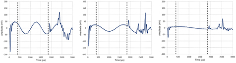
Figure 3. Example waveforms acquired during the calibration of the TC 4032 hydrophone in the NPL open tank facility for acoustic drive frequencies of 1 kHz, 750 Hz and 400 Hz. Clearly visible are the start-up transients caused by the projector, and the arrival of the acoustic reflections after about 2 ms. The dashed lines indicate the time windows used to select the steady-state signal.
Download figure:
Standard image High-resolution imageThe ability to reach steady-state conditions depends on the available echo-free time, which is governed by the geometry of the tank and position of transducers and does not change for each frequency of excitation.
If τ is the echo-free time for a particular tank and transducer locations, the number of echo-free cycles available for analysis is equal to the product ντ where ν is the frequency of excitation. For resonant electroacoustic devices of quality factor Q, it takes Q cycles of the resonance frequency for the signal to reach approximately 96% of its final steady-state value (so that the initial turn-on transients have almost completely died away). The same resonant behaviour occurs for all frequencies of excitation, even where the projector is driven off-resonance. For situations where Q > ντ, steady-state is not reached and it is not possible to make a direct measurement of the steady-state signal by conventional means.
Figure 4 shows the results of the calibrations of the Reson TC 4032 hydrophone and the B&K 8104 hydrophone measured by the free-field three-transducer reciprocity method and by the pressure calibration method of comparison in a closed chamber. Shown in the plots are the sensitivity level measured by the method of three-transducer reciprocity, with the amplitude of the steady-state part of the signals during the calibration determined by the simple least-squares fitting technique. The circles display the sensitivity of the hydrophone as determined by comparison to a reference microphone in a closed chamber. The error bars shown indicate the uncertainties for a coverage factor of k = 2 [42]. A discussion of the sources of uncertainty is provided in section 5.

Figure 4. Sensitivities of the Reson TC 4032 hydrophone (left) and the B&K 8104 hydrophone (right) measured by the free-field three-transducer reciprocity method using the signal-modelling (squares) and by pressure calibration method of comparison in a closed chamber (circles). The error bars show the expanded calibration uncertainties expressed for a coverage factor of k = 2.
Download figure:
Standard image High-resolution image4.2. TVR of high-Q low frequency projector
Figure 5 shows example waveforms acquired during the calibration of the 2 kHz flexural-disc transducer showing signals acquired in the APV (solid blue curve) where the signal recorded is contaminated by reflections arriving at a time of approximately 2 ms (denoted by the arrows), and at the open-water facility where the steady-state signal can be observed in free-field conditions (dashed red curve). In the case of the signal acquired in the APV facility, it is impossible to observe the steady-state signal directly within the available echo-free time, whereas the steady-state is seen fully established after about 6 ms in the signal from the open-water facility.
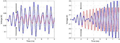
Figure 5. Example waveforms acquired during the calibration of the 2 kHz flexural-disc transducer at frequencies of 1.5 kHz (left) and the resonance frequency of 2 kHz (right). The blue waveforms (solid) are the signals acquired in the APV, and the red waveforms (dashed) are those obtained in at the open-water facility. The arrows denote the arrival of the first reflection in the case of the APV measurements.
Download figure:
Standard image High-resolution imageFigure 6 shows the model fit (dashed red curve) for measured data (solid green curve) for the example of the 2 kHz transducer driven at 1.5 kHz. Those parts of the waveforms within a time-window lasting about 1.8 ms are treated by the technique (about twice the echo-free time and half the total acquisition time). The fitted model assumes two reflections of the transmitted signal (marked by the vertical dashed lines). For purposes of illustration, the time of arrival of the transmitted signal is defined to be time origin t = 0.

Figure 6. Model fit (dashed red curve) for measured data (solid green curve) for the 2 kHz hydrophone driven at 1.5 kHz. Those parts of the waveforms within a time-window lasting about 1.8 ms are treated (about twice the echo-free time and half the total acquisition time). The fitted model assumes two reflections of the transmitted signal (marked by the vertical dashed lines).
Download figure:
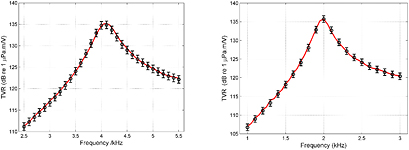
Standard image High-resolution imageFigure 7 shows the results of the calibration for the 4 kHz and 2 kHz high-Q devices respectively. The continuous curve shows the TVR obtained from analysing the steady-state part of the waveforms measured at the NPL open-water facility. The circles show the estimates obtained by applying the signal modelling method to analyse the waveforms obtained in the APV. Those parts of the waveforms restricted to a time-window lasting 1.8 ms have been treated. The model used includes two resonances and two reflections of the transmitted signal. The error bars illustrate the (k = 2) expanded uncertainties associated with the estimates from the signal modelling method. The uncertainties from the free-field measurements are not shown, but these are approximately 1 dB at all frequencies.
Figure 7. The measured TVRs for the 4 kHz projector (left) and 2 kHz projector (right) showing the free-field results from the open-water facility (solid curve), and the results of signal modelling applied to the waveforms measured in the APV (circles with associated k = 2 expanded uncertainties shown as error bars).
Download figure:
Standard image High-resolution image
5. Discussion
5.1. Uncertainty evaluation for fitting process
The uncertainty matrix (covariance matrix) U associated with the solution is given, formally, by

where u(y) is the standard uncertainty associated with the measured values yil, and J is a matrix containing the derivatives of eil with respect to the model parameters evaluated at the solution. The diagonal elements of U are the variances (squared standard uncertainties) associated with the estimates of the model parameters. The off-diagonal elements are the covariances associated with pairs of parameters. An a posteriori estimate of u(y) is provided by
with S2 is evaluated at the solution and n the number of model parameters.
An application of the law of propagation of uncertainty is used to evaluate the standard uncertainty associated with an estimate of the amplitude Ai of the steady-state response [42]. Based on a first order approximation,
where the variances u2(Ci00) and u2(Si00), and covariance u(Ci00, Si00), are elements of U.
A further application of the law of propagation of uncertainty is used to evaluate the standard uncertainty associated with an estimate of the transmitting voltage response, i.e.

where the quantities in the model for  are assumed to be independent.
5.2. Other sources of uncertainty
The sources of uncertainty in the free-field calibration methods are described in the scientific literature including IEC 60565:2006 [2], and they are not repeated in detail here. They include the calibration uncertainty in the reference hydrophone used for the determination of the TVR (described in section 3.2), the separation distance between source and receiver, and for the reciprocity calibration method, the assumption that at least one device is reciprocal. The major sources of uncertainty at low kilohertz frequencies are caused by the lack of steady-state conditions (mitigated by the advantages of the signal modelling method), and poor signal-to-noise ratio.
The uncertainty in the hydrophone calibration method is influenced by electrical noise exacerbated by the roll-off in transmitting response of projectors used in the calibration, which typically exhibit a quadratic dependence on frequency (12 dB per octave) well below resonance, leading to very low sound pressures in the water during calibrations at frequencies below 1 kHz. One solution is to use a source transducer with a higher transmitting response, increasing the signal level, but such a device would have a resonance at a lower frequency leading to start-up transients of longer duration (reducing the steady-state signal available for analysis). The effect of broadband electrical noise can be reduced by coherent time averaging of the time waveforms. To test the effect of noise on the fitting process, example noisy waveforms were synthesised with a signal frequency of 250 Hz and 5% noise amplitude. Using a time window of 1 ms (equivalent to one quarter of a cycle), the uncertainty on amplitude with no averaging was as high as 1.5%, but when at least 10 averages were used for the waveform acquisition, the uncertainty reduced to less than 0.5 %.
Interference from a coherent signal of a specific frequency cannot be removed by coherent averaging. However, if the interference is at a significantly higher frequency, the influence on the fitted amplitude will not be severe. Using synthesised waveforms with a signal frequency of 250 Hz and an added signal of 5 kHz at 10 % amplitude, analysis of one quarter of a cycle led to an amplitude uncertainty of less than 1 %. However, interference at a frequency close to the signal drive frequency can have a more significant effect. In the work reported here, particular problems were found with electrical interference at harmonics of the electrical supply frequency causing fluctuations at 250 Hz, leading to degraded repeatability in calibrations at this frequency. Although the problem was mitigated by careful shielding, use of battery-operated and low-noise instrumentation, there remained some residual effects which increased the uncertainty at this frequency.
At these low frequencies, the slope of the transmitting response of the projectors used will cause any harmonic distortion in the drive signal to be amplified. Any distortion in the signal due to overdriven transducers or harmonic distortion in the electrical drive signal will lead to errors in the fitting process, and should be avoided. However, since the definition of transmitting response assumes linear behaviour in any case, this issue is common to any calibration method, including the traditional procedures.
The extended method can include the initial reflected signals as part of the signal to be modelled. In this case, the transducer transmitting response may be modified by the presence of the reflected signals through the radiation impedance of the transducer. This adds to the uncertainty for a high Q-factor device at frequencies close to resonance, where the transducer is most sensitive to the medium impedance, and will be more important for transducers where the radiation impedance is a significant proportion of the transducer impedance. For the flexural-disc projectors calibrated here, the comparison with the true free-field response measured at the open-water facility did not show significant bias in the results which may be attributed to this effect.
5.3. Advantages and limitations
The amplitude (and phase) of signals used in calibrations may be determined in a number of ways, including by the use of Fourier techniques [2]. The advantage of fitting a sinusoidal function to the windowed waveform is that the method has no requirement for an integer number of cycles within the window, may be used on short segments of waveform (even on a fraction of one cycle of the waveform), and the method is relatively robust against noise. If the sampling frequency is much greater than the measurement frequency, as will generally be the case for the low frequencies used here, the averaging effect of the least-squares fit means that reliable estimates of the signal amplitude can be produced even when the measured waveform segment is noisy.
For the simple method, the method is relatively easy to implement and maintains true free-field conditions (unlike methods which are undertaken in reverberant conditions) while extending the frequency range downward by up to two octaves. The limitations on the use of the simple method depend on the available echo-free time and the Q-factor of the projector, but also the frequency of the projector resonance. For a given Q-factor, using a projector which has a lower resonance frequency will in general increase the amount of echo-free time lost to the transient signal (which lasts for a greater duration if the resonance frequency is lower). The simple method may be used in situations where at least one quarter of a cycle of signal is available free of echoes and transients. Note that the transient behaviour observed in the signal will also depend on the Q-factors of other items in the measuring system. If the receiving hydrophone has a resonance close to the frequency of measurement, this will influence the waveform shape, as will any measuring instrument (amplifier, filter, etc) which displays any resonant behaviour in the frequency range.
Once the steady-state signal is no longer observable at all, the extended modelling method provides the possibility to estimate the amplitude (and phase) from segments of the waveform which would be unusable for traditional calibration techniques. The method depends on the assumption that the transducer may be modelled as a lumped-parameter harmonic oscillator. Though this is valid for many simple piezoelectric hydrophones and transducers at frequencies close to and below resonance, this assumption can be invalid for more complex designs of transducer. The method is also more difficult for transducers which exhibit strongly-coupled resonances which are close in frequency, as can be the case for some ring transducers.
The extended method enables the calibration of challenging high Q-factor projectors and does not suffer from some of the difficulties of other methods, such as the reliance on the acoustic properties of the test tank in producing a reverberant acoustic field, and it can be implemented with high drive levels (a difficulty with some transient-suppression methods). The extended method benefits from both increasing the time length for analysis (into the reflected signals) and analysing all signal frequencies simultaneously (and making use of the fact that the resonance phenomena are common to all signals), and each of these has been studied in detail in the NPL technical reports referenced [33].
One difficulty in the extended modelling approach is the choice of good starting estimates for the model parameters. Obtaining estimates of resonance frequencies and damping factors from electrical impedance measurements is relatively straightforward and accurate [1, 3, 13]. In this work, estimates for the echo arrival times were obtained from consideration of the geometry of the laboratory tanks. If such estimates are not available, other signal processing may be used to estimate the arrival time without a priori information. Signal processing techniques such as wavelet analysis may also be useful for empirically extracting information about the arrival times from the measured data [43].
6. Conclusions
This paper has described the application of a signal modelling method for the calibration of both hydrophones and high-Q projectors in the range 250 Hz–5 kHz. For hydrophones exhibiting a low-Q response, a linear least-squares fit of a sinusoidal signal to short segments of the acquired waveforms enables extension of the traditional calibration techniques down to frequencies well below the typical low-frequency limit for such calibrations. Results have been presented of calibration of two reference hydrophones using this method, with good agreement to pressure calibrations undertaken in a small coupler.
In the extended method, the response of a device is modelled by a function consisting of a sum of terms that describe the steady-state and resonant behaviour of the device(s), with the model describing the response both to the direct signal and to reflections of the signal from the tank boundaries. A non-linear least-squares method has been used to provide improved estimates of the model parameters and results are presented for calibrations undertaken in a modest-sized pressure vessel on two flexural disc transducers with resonance frequencies of 2 kHz and 4 kHz and Q-factors of 10. The calibrations were validated by comparison with measurements made under the same conditions at an open water facility, where it was possible to undertake measurements under steady-state conditions. Excellent agreement was obtained with results agreeing to within 1 dB, well within expanded uncertainties.
The signal modelling method has the potential to extend the frequency range downward for calibrations for electroacoustic transducers, including high-Q projectors by up to an order of magnitude in frequency for a laboratory tank of modest size. The technique enables the user to maximise the frequency range of measurements made in laboratory tanks where greater environmental control is available, and minimises the need for use of large deep-water facilities, which can be expensive, logistically difficult to operate, and offer little control of the environment.
Acknowledgments
The authors acknowledge the support of the UK's Department of Business, Energy and Industrial Strategy.