


Abstract
Saline solutions are of a great interest when characterizations of biological fluids are targeted. In this work a near-field microwave microscope is proposed for the characterization of liquids. An interferometric technique is suggested to enhance measurement sensitivity and accuracy. The validation of the setup and the measurement technique is conducted through the characterization of a large range of saline concentrations (0–160 mg ml−1). Based on the measured resonance frequency shift and quality factor, the complex permittivity is successfully extracted as exhibited by the good agreement found when comparing the results to data obtained from Cole–Cole model. We demonstrate that the near field microwave microscope (NFMM) brings a great advantage by offering the possibility to select a resonance frequency and a quality factor for a given concentration level. This method provides a very effective way to largely enhance the measurement sensitivity in high loss materials.
Export citation and abstract BibTeX RIS
1. Introduction
Conventional microwave characterization tools based on resonant cavities, waveguides, open-ended coaxial lines and free space methods have shown some potentials for the characterization of various materials [1–6]. Nevertheless a major drawback of these techniques is that their measurement sensitivity falls in the presence of high-loss media such as liquids [7, 8]. Also, many conventional approaches involve samples whose size is in the order of tens of square millimeters in terms of surface [9, 10]. More recently, near-field microwave microscopy (NFMM) has demonstrated great advantages for numerous emerging applications especially for liquids sensing [11, 12]. Thanks to its high spatial resolution, the NFMM enables a very local characterization of materials properties [13–15]. In fact the spatial resolution is mainly governed by the probe apex size. However, one big challenge of the NFMM is to overcome the impedance mismatch problem between the microwave source (i.e. a 50 Ω impedance network analyzer) and the evanescent microwave probe (EMP) whose impedance is in the order of kΩ [11, 12, 16, 17]. As a result, to solve the measurement sensitivity issue induced by this impedance difference, a matching network has been integrated in-between this 2 parts of the NFMM system [18, 19].
Usually, there are two approaches to match the VNA to probes: the resonant and interferometric methods. Nevertheless, the operating frequency band is very limited for the resonator-based NFMM. Moreover, the measured quality factor provided by the instrument falls a lot in the presence of high loss materials such as liquids no matter how high the quality factor is in free space [20]. This problem makes it hard for resonator-based microscopes to perform some important applications in liquid environment like for the example in biological fluids. Because of the resulting poor measurement sensitivity, this approach is not the best suited and so the interferometry one is preferred for this kind of applications [19, 21].
From this observation, in this work a NFMM platform based on an interferometric technique is exploited to characterize liquid solutions. We demonstrate in which extent the interferometer-based microscope enables characterizations in a broad frequency range (2–18 GHz) with high measurement sensitivity and accuracy. The choice of saline aqueous solutions as the liquid under test is motivated by the fact that it is quite easy to obtain samples with calibrated concentrations and also because the saline aqueous solutions are used very commonly to simulate biological fluids [22, 23]. As a result, there is a great motivation in developing precise tools to investigate NaCl concentrations in aqueous solutions. In this paper, a brief description of the microscope configuration is given in section 2. In section 3, based on the Cole–Cole model, dielectric properties are theoretically studied for the entire NaCl concentration range considered (0–160 mg ml−1) with a focus on concentrations included in (0–9 mg ml−1). Actually, the normal saline (NS) concentration level of biological tissues fluid is around 9 mg ml−1 [22, 24], so, there is a special interest for this range of concentration. In section 4, the electric field distributions of the microwave probe in NaCl solutions with different concentrations are demonstrated by electromagnetic simulations. In section 5, the high measurement sensitivity and accuracy brought by the interferometric technique is validated by experimental results. Finally in the last section, a model is proposed to relate the complex permittivity to the measured resonance frequency shift and quality factor. Additionally, the influence of the reference concentration on the measurement sensitivity and precision is carefully studied.
2. Near-field microwave microscope configuration
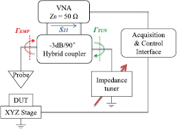
The architecture of the microwave microscope is depicted in figure 1. To achieve a broad frequency range operation and a high measurement accuracy, the interferometer is built up with a hybrid coupler and an impedance tuner including a high-resolution programmable delay line and a motor-driven variable attenuator.
Download figure:
Standard image High-resolution imageThe hybrid coupler is connected to the ports 1 and 2 of the vector network analyzer (VNA). The direct and coupled paths are connected to the EMP (with reflection coefficient ΓEMP) and to the impedance tuner (with reflection coefficient ΓTUN) respectively. In this configuration, the coupler has two functions. First, it acts as a reflectometer that separates the incident signal from the one reflected by the EMP. Secondly, by combining the waves coming respectively from the probe and the impedance tuner, it gives the possibility to tune the resulting signal to a very low level. Particularly, ΓTUN is carefully adjusted to compensate ΓEMP by adequately choosing attenuator and phase-shifter positions that lead to a signal with an equal magnitude and an opposite phase-shift when comparing to ΓEMP. This combined signal is called zero level signal. Actually, this signal is measured in a transmission mode (S21) to overcome the main limitation encountered when using VNAs, in terms of directivity errors, especially on the measurement of small signals. Thus, the technique gives the possibility to operate in the ultimate sensitivity range of the VNA.
As shown in figure 1, the device/material under test to be measured is mounted on a x–y–z stage. The probe is positioned vertically over the stage. The stage consists of three independent motorized linear translation sub-stages with respectively travel distances of 25 cm in x/y axis and 1 cm in z axis. The minimum increment step in the three directions is 1 µm. Furthermore, the sample is positioned on the chuck fixed on the stage to allow, in case of scanning tests, a displacement in the three axis whereas the microwave part of the microscope remains fixed to lower the electrical errors due to the RF cables movements. More information on the instrumentation can be found in [11, 12].
In the following section, dielectric properties of saline solutions are theoretically studied by using the Cole–Cole model.
3. Complex permittivity determination from Cole–Cole model
It is well acknowledged that the permittivity of materials expresses their ability to polarize in response to an applied field and can be written as:

where  is the complex permittivity,
  and
and  are the real and imaginary part of the permittivity respectively, and
  is the loss tangent of permittivity. Cole–Cole equation [24, 25] can be expressed by:
where  and
and  are respectively the limit of the permittivity at high and low frequencies,
  is the ionic conductivity,
  is the relaxation time,
  is a distribution parameter and
  is the permittivity of free space. After the calculation of all these parameters (
 ,
,  ,
,  ,
,  and
and  ) at 25 °C, the complex permittivity can be determined. As a demonstration, the results for saline concentrations ranging from 0 to 160 mg ml−1 (0–2.74 mol l−1) are presented in figure 2(a) for a frequency of 2 GHz. Additionally, as the normal saline concentration of biological tissues fluid is in the order of 9 mg ml−1, the responses at 2 GHz in the range (0–9 mg ml−1) are also presented in figure 2(b). The concentration 0 mg ml−1 represents deionized water (DI water).
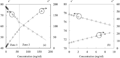
Figure 2. Complex permittivity of saline solutions based on Cole–Cole model at 2 GHz; (a) NaCl concentration range from 0 to 160 mg ml−1; (b) NaCl concentration range from 0 to 9 mg ml−1; T = 25 °C, F0 = 2 GHz.
Download figure:
Standard image High-resolution imageAs shown in figure 2(a), the real part of the permittivity (dielectric constant) decreases from 78 to 50 in the concentration range (0–160 mg ml−1), while in the same range, the imaginary part of the permittivity (dielectric loss) increases from 7 to 170. Furthermore, one can note that the results of the complex permittivity exhibit linear behaviors as a function of the NaCl concentrations. Indeed, two linear zones can be identified in figure 2(a): zone 1 for concentrations lower than 58 mg ml−1 (1 mol l−1), and zone 2 for concentrations higher than 58 mg ml−1. Thus, for saline concentrations in the range (0–58 mg ml−1) (figure 2(a)), the real and the imaginary part of the permittivity can be described by the following equations:


where C represents the concentration of sodium chloride. In the same way, the complex permittivity for concentrations ranging in (58–160 mg ml−1) can be expressed by:
On the other hand, the results for NaCl concentration spreading from 0 to 9 mg ml−1 are presented in figure 2(b). In this case, the dielectric constant slightly decreases from 78 to 76, while in the same range, the imaginary part of the permittivity increases from 7 to 20. As this range is part of the zone 1, the complex permittivity is also governed by equations (1) and (2).
Thanks to these linear equations, the complex permittivity around 2 GHz can be easily evaluated for any NaCl concentrations ranging from 0 to 160 mg ml−1. Furthermore, the knowledge of the complex permittivity allows simulations to investigate the electromagnetic response of NaCl solutions by means of commercial software, such as ANSYS/HFSSTM.
4. Electromagnetic simulation of the probe-sample interaction
The probe-sample interaction is first numerically studied by using the electromagnetic simulation software, ANSYS/HFSSTM. The probe is made of a coaxial line whose central metallic conductor is extruded and ended by a semi-sphere (diameter: 260 µm). The simulation data entries for the liquid (ε' and ε'') are determined from the Cole–Cole equation (see section 3). As a demonstration, four saline concentrations are considered in the simulation: two solutions (0 mg ml−1 and 9 mg ml−1) in the linear zone 1 (C < 58 mg ml−1), and two others (80 mg ml−1 and 160 mg ml−1) in the linear zone 2 (C > 58 mg ml−1). Figure 3 shows the distribution of the electric field magnitude at the cross section along the probe. For these simulations the probe tip is immersed in the liquid solution at a depth of 300 µm and the test frequency is 2 GHz.
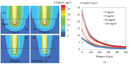
Figure 3. Simulation (ANSYS/HFSSTM) of the microwave probe (apex = 260 µm) electric field magnitude for different saline concentration levels: (a) 0 mg ml−1, (b) 9 mg ml−1, (c) 80 mg ml−1 and (d) 160 mg ml−1, (e) E-field as a function of the distance H from the tip; probe immersed in liquid at a depth of 300 µm; T = 25 °C, F0 = 2 GHz.
Download figure:
Standard image High-resolution imageFigure 3 points out clearly that the simulated electrical field decays rapidly with the distance to the probe. As the electric field around the probe apex is much stronger than elsewhere (figures 3(a)–(d), as already said, a local characterization of materials can be achieved [22, 26]. The spatial resolution in this study is in the order of 260 µm (probe apex size). The corresponding maximum E-field value varies with the saline concentrations. Actually, as shown in figure 3(e), the E-field decays rapidly with the distance to the probe and its maximum diminishes with the concentration (27, 25, 14 and 8 V mm−1 respectively for 0, 9, 80 and 160 mg ml−1). Indeed, the saline solutions absorb more electric energy generated by the microwave probe when the NaCl concentration level increases and the E-field penetration falls when the liquid becomes more conductive. For example when the E-field falls down from its maximum to 5 V mm−1, the corresponding distance to the probe are 196, 192, 87, 66 µm respectively for 0, 9, 80 and 160 mg ml−1 (figure 3(e)). When the concentration is increased, the distance is shortened.
After the simulation study of the probe-liquid interaction, the microwave responses of the proposed NFMM are experimentally validated in the following section. To demonstrate the performance of the interferometer-based microwave microscope, we compare the resulting measurement sensitivity with the value obtained when using the instrument without the interferometer setup.
5. Evaluation of the measurement sensitivity
In this section, the response of the microwave microscope is experimentally evaluated. A plastic container (7.4 × 7.4 × 5.4 mm3) is used to hold the liquid solutions under test. The setting parameters of the VNA are 2 GHz for the frequency, 0 dBm for the power and 100 Hz for the intermediate frequency bandwidth (IFBW). The probe with apex of 260 µm is employed for the liquid characterization. As shown in the section 4, the microwave probe has potentials for local characterization as the E-field is well confined around the tip apex. During the measurement, the probe is immersed at a depth of 300 µm in the liquid ensuring the whole tip apex is plunged in liquid under test. Thus a maximum tip-liquid electromagnetic coupling can be obtained. Another advantage in case of an immersed probe is the immunity to water evaporation process at the liquid surface layer which can largely influence the air-liquid interface and the concentration of saline solutions.
As already mentioned, two configurations are considered: without interferometer (inset of figure 4(a): reflection mode) and with interferometer (figure 1: transmission mode). To evaluate the measurement sensitivity provided by these two working modes, low saline concentration levels, (0–9 mg ml−1), are considered as the fluids under test. The choice of this NaCl solution concentration range is also motivated as already said by the fact the 9 mg ml−1 saline concentrations level represents an essential component of the biological fluids. Thus, figure 4 presents the measured microwave responses of saline concentrations from 0 to 9 mg ml−1 in the frequency band (1.996–2.004 GHz). Actually, for the reflection mode the probe is connected directly to one port of the VNA without the impedance tuner and the coupler in-between (inset of figure 4(a)). In this configuration, the reflection coefficient S11 is acquired.

Figure 4. Measured reflection coefficient S11 of different saline solutions from 0 mg ml−1 to 9 mg ml−1; (a) magnitude plot, (b) phase-shift plot; F0 = 2 GHz; P0 = 0 dBm; IFBW = 100 Hz, T = 25 °C [27].
Download figure:
Standard image High-resolution imageAs shown in figure 4, the instrument without interferometer can distinguish the different saline concentrations from 0 to 9 mg ml−1 but with limited sensitivity. Indeed, in figure 4(a), between the concentration limits (0 and 9 mg ml−1), a variation of magnitude smaller than 0.5 dB is noticed at 2 GHz. Meanwhile, in figure 4(b), a variation around 5° between these two saline concentrations is observed. Thus, the results collected by using this configuration return a measurement sensitivity of 0.06 dB/(mg/ml) and 0.6 °/(mg/ml) for magnitude and phase-shift respectively.
After the analysis of the instrument without interferometer, we present now the results for the system with interferometer. In this case, thanks to the impedance tuner made of variable attenuator and delay line, the tip is preliminary matched in DI water (0 mg ml−1) by tuning |S21| to −55 dB (35 dB above the noise floor of the VNA which is −90 dB) at 2 GHz. As described before, this level represents the zero level after combining the wave reflected by the probe and the wave generated by the impedance tuner (figure 1). The saline solutions from 1 to 9 mg ml−1 are then sequentially measured and their responses in terms of transmission coefficient (S21) magnitude and phase-shift are collected in figure 5.
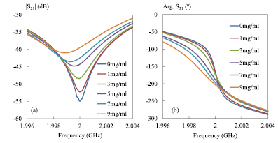
Figure 5. Measured transmission coefficient S21 for different saline solutions from 0 mg ml−1 to 9 mg ml−1; (a) magnitude plot, (b) phase-shift plot; 0 mg ml−1 (DI water) = reference value; F0 = 2 GHz; P0 = 0 dBm; IFBW = 100 Hz; zero level = −55 dB, T = 25 °C [27].
Download figure:
Standard image High-resolution imageAs demonstrated in figure 5, the interferometer-based method can easily distinguish small saline concentrations from 0 mg ml−1 to 9 mg ml−1 with high measurement sensitivity. We obtain at 2 GHz a maximum variation of the magnitude and the phase-shift around 14.1 dB (figure 5(a)) and 35.7° (figure 5(b)) respectively, which is much higher than the values obtained by the instrument without interferometer. To better appreciate the measurement sensitivity offered by the two working modes, we summarize the sensitivity values in table 1.
Table 1. Measurement sensitivity to saline concentration levels from 0 to 9 mg ml−1 with the two configurations considered: without interferometer (reflection mode) and with interferometer (transmission mode); F0 = 2 GHz; P0 = 0 dBm; IFBW = 100 Hz.
| Without interferometer | With interferometer | |
|---|---|---|
| Magnitude | Δ |S11| = 0.06 dB/(mg/ml) | Δ |S21| = 1.56 dB/(mg/ml) |
| Phase-shift | Δ arg. S11 = 0.6 º/(mg/ml) | Δ arg. S21 = 3.9 °/(mg/ml) |
As shown in table 1, the measurement sensitivities reached when using the interferometer, 1.56 dB/(mg/ml) and 3.9°/(mg/ml) for magnitude and phase-shift respectively, are clearly much higher than the measurement sensitivities provided by the configuration without interferometer. Therefore, thanks to the interferometric technique, the proposed NFMM is able to precisely detect a very small variation of the saline concentration. Particularly, by using the impedance tuner, resonances with high quality factors are acquired. By contrast, in the no-interferometer case (figure 4(a)), no resonance can be found due to the poor measurement sensitivity. Additionally, it can also be observed in figure 5(a) that the resonance peak of |S21| shifts to the left side (low frequencies) as the saline concentration level increases. So, a shift of the resonance frequency from the resonance frequency observed for the reference level can be evaluated for each concentration even for very small variations.
These results are the basis of the method for the determination of the dielectric properties of the liquid samples tested. Actually, the complex permittivity can be quantified from the knowledge of the resonance frequency shift (ΔF) and the quality factor (Q) of |S21| [28]. The different steps for this determination are presented in the next section.
6. Extraction of the complex permittivity of saline solutions
Based on figure 5(a), the resonance frequency shift (ΔF) and the quality factor (Q) of the measured |S21| are given in figure 6. In fact, ΔF represents the difference between the resonance frequency of the saline concentration considered (Fmeas) and the value (F0) registered for DI water (reference solution):

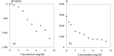
Figure 6. Resonance peak parameters obtained from the measured transmission coefficient |S21| as a function of saline concentration; (a) resonance frequency shift ΔF; (b) quality factor Q, 0 mg ml−1 represents reference value; F0 = 2 GHz; P0 = 0 dBm; IFBW = 100 Hz; zero level = −55 dB.
Download figure:
Standard image High-resolution imageFor DI water, the corresponding F0 is 2 GHz and Q0 is around 2900. Thus, the resonance frequency shift ΔF and Q factor of saline concentrations from 0 to 9 mg ml−1 are presented in figure 6.
As shown in figure 6(a), the resonance shift increases with the concentration level and the maximum shift is around 1200 kHz. On the other hand, it is observed in figure 6(b) that the quality factor decays as a function of the concentration. In particular, the maximum Q value (2900 obtained at 0 mg ml−1—reference) decreases to 600 for a solution at 9 mg ml−1, representing a reduction of almost a factor 5.
According to [29], the resonance shift ΔF is closely related to the variation of the dielectric constant ε' while the fall of the quality factor represents the variation of dielectric loss ε'' of the material under test. The relation between the ΔF, Q and the complex permittivity can be expressed as:

Based on figure 6, the quantities ΔF/F0 and Δ(1/Q) measured as a function of saline concentration are given in figure 7.
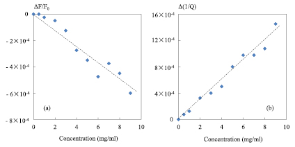
Figure 7. Resonance peak parameters obtained from the measured transmission coefficient |S21| as a function of saline concentration; (a) ΔF/F0; (b) Δ(1/Q); dashed lines represents fitted polynomial line at first order, 0 mg ml−1 represents reference value; F0 = 2 GHz; P0 = 0 dBm; IFBW = 100 Hz; zero level = −55 dB.
Download figure:
Standard image High-resolution imageAs shown in figure 7, ΔF/F0 and Δ(1/Q) are practically proportional to the NaCl concentration level. So, the behavior of ΔF/F0 and Δ(1/Q) can be expressed as a function of saline concentration (C) by those equations:

A' and A'' represent the slopes of the fitted polynomial line in figures 7(a) and (b), respectively. Thus we obtain A' = −6.25 × 10⁻⁵ ml mg−1 and A'' = 1.48 × 10⁻⁴ ml mg−1. With these two parameters, the measured ΔF/F0 and Δ(1/Q) are mathematically related to the saline concentration levels. In addition, thanks to the relations linking the complex permittivity and the NaCl concentrations discussed in section 3, the measured ΔF/F0 and Δ(1/Q) can be related to the saline solutions complex permittivity by the following equations:
One can note that instead of using a fitting model, a simpler and faster calibration method consists in just selecting as calibration standards the limits of the concentration range investigated (i.e. 0 and 9 mg ml−1 in this case).
After the calibration process, the measured complex permittivity in the concentration range (0–9 mg ml−1) is then obtained. For comparison, the theoretical values calculated from Cole–Cole model are also presented in figure 8.
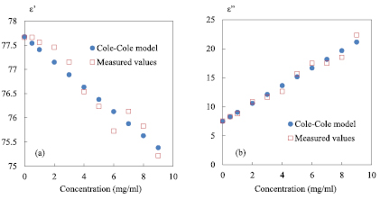
Figure 8. Complex permittivity as a function of saline concentration; (a) dielectric constant ε'; (b) dielectric loss ε''; round symbols = values based on the Cole–Cole model, square symbols represent measured values; 0 mg ml−1 represents reference value; F0 = 2 GHz; P0 = 0 dBm; IFBW = 100 Hz; zero level = −55 dB.
Download figure:
Standard image High-resolution imageThis figure exhibits a good agreement between the theoretical and experimental complex permittivity at 2 GHz for the saline concentration range (0–9 mg ml−1). Thus, one can conclude thanks to the equations (5) and (6) that the measured complex permittivity is successfully extracted. Actually, these equations remain available for the concentrations range (0–58 mg ml−1) (linear zone 1 of figure 2(a)) and equivalent treatment can be applied by using them. The method based only on two known concentrations has also been checked. Even if the results are a little bit different, they remain comparable and acceptable. In case of field measurements it is an option to consider. Concerning the linear zone 2 (figure 2(a)), a similar extraction method based on ΔF/F0 and Δ(1/Q) can be used and a new set of equations is established. The results are gathered to represent the complex permittivity on the entire range of concentrations from 0 to 160 mg ml−1 in figure 9.
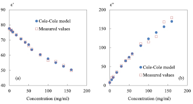
Figure 9. Complex permittivity as a function of saline concentration; (a) dielectric constant ε'; (b) dielectric loss ε''; round symbols represent values based on the Cole–Cole model, square symbols represent measured values; 0 mg ml−1 represents reference value; F0 = 2 GHz; P0 = 0 dBm; IFBW = 100 Hz; zero level = −55 dB.
Download figure:
Standard image High-resolution imageAs shown in figure 9(a), a good agreement is found between the permittivities calculated by the Cole–Cole model and the measured ones for such a large NaCl concentrations range spreading from 0 to 160 mg ml−1. To investigate the measurement precision, the difference between measurement and theory for each concentration from 0 to 160 mg ml−1 is calculated and the average over the set of values is then computed. In this case, the averaged error is in the order of 1.6% and 8% for ε' and ε'', respectively. Higher discrepancy is noticed for the high concentrations from around 100 mg ml−1 (figure 9(b)). A way to increase the measurement sensitivity and precision in the upper range of concentrations is to consider as a reference value a higher concentration instead of 0 mg ml−1 (DI water). As a demonstration, 3 other concentrations are considered as the reference solution: the maximum concentration level (160 mg ml−1) and two medium concentrations (58 and 100 mg ml−1). For the setting parameters of the VNA, the operating frequency is kept at 2 GHz, 0 dBm for the power and 100 Hz for IFBW. The probe is still immersed at a depth of 300 µm in the liquid under test. The zero level of |S21| is tuned to −55 dB for the reference solutions. In figure 10, we give the measured quality factor for the 4 reference solutions selected: 0, 58, 100 and 160 mg ml−1.
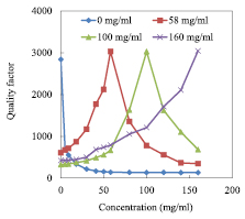
Figure 10. Quality factor as a function of saline solutions considering different reference solutions: 0, 58, 100 and 160 mg ml−1; F0 = 2 GHz; P0 = 0 dBm; IFBW = 100 Hz; zero level = −55 dB.
Download figure:
Standard image High-resolution imageIt can be noted from figure 10 that the quality factor for the reference solution remains relatively stable around 3000, which means a high measurement sensitivity is obtained for these concentrations. This possibility of tuning the quality factor as a function of concentration is one of the main assets of the NFMM proposed, in particular when liquids are investigated. In the following, we evaluate the impact of the reference concentrations on the measured permittivity (figure 11).
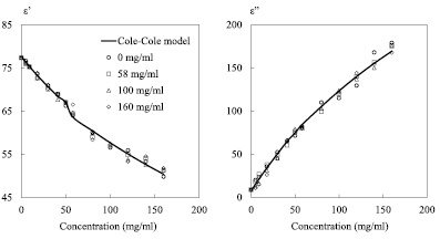
Figure 11. Complex permittivity for 4 NaCl reference concentrations: 0, 58, 100 and 160 mg ml−1; (a) dielectric constant ε'; (b) dielectric loss ε''; solid lines represent values based on the Cole–Cole model, symbols represent measured values; zero level is −55 dB for the 4 reference concentrations; F0 = 2 GHz; P0 = 0 dBm; IFBW = 100 Hz.
Download figure:
Standard image High-resolution image
Generally speaking, the measured permittivity is in a good agreement with the values based on Cole–Cole model for the entire concentration range (0–160 mg ml−1) whatever the reference concentration is. Nevertheless, one can note that the reference concentration levels influence to some extent the measured permittivity values. For example, in figure 11(b), for a given NaCl concentration such as 120 mg ml−1, the theoretical value ε'' is 140 whereas the measured results 129, 136, 135 and 143 retrieved when using the 4 reference concentrations (0, 58, 80 and 160 mg ml−1) respectively. These results show that especially for ε'' the difference between the measured value and the theoretical data is enlarged when the tested solution presents a concentration that is moved away from the reference solution. Thus, the measurement quality of the complex permittivity is closely associated to the reference concentration level. To better appreciate the relation between the reference concentrations and the measurement results, we summarize in table 2 the averaged error calculated from the difference between the measured permittivities and the theoretical values for each concentration for the 4 cases envisaged (reference level = 0, 58, 100, and 160 mg ml−1).
Table 2. Averaged errors in percentage for different reference concentration levels (0, 58, 100 and 160 mg ml−1); F0 = 2 GHz; P0 = 0 dBm; IFBW = 100 Hz; zero level = −55 dB.
| 0 mg ml−1 | 58 mg ml−1 | 100 mg ml−1 | 160 mg ml−1 | |
|---|---|---|---|---|
| ε' (%) | 1.6 | 0.9 | 0.9 | 1.6 |
| ε'' (%) | 7.8 | 7.0 | 7.1 | 8.5 |
As shown in table 2, the maximum averaged error reported is 1.6% and 8.5% for the real and imaginary parts of the permittivity, respectively. One can also note that a lower error is obtained for both ε' and ε'' for reference concentrations at 58 and 100 mg ml−1. This result confirms that a better measurement precision can be found when the reference concentration is not taken at the limit of range investigated. Thus, to guarantee a precise measurement, the intermediate concentrations (e.g. 58 and 100 mg ml−1) should be preferentially selected as reference concentrations instead of the minimum (0 mg ml−1) or maximum concentrations (160 mg ml−1). Actually, thanks to the interferometer which is equipped with variable attenuator and delay line, high measurement sensitivity can be easily guaranteed at any desired reference concentrations. So, it is relatively simple to choose for example the middle of the range of interest as the reference concentration level.
Finally, thanks to the good standard deviation offered by our platform, less than 1% [30], we obtain permittivities values that agree very well with those retrieved by the standard coaxial method but with a volume under test much smaller.
7. Conclusion
The characterization of the complex permittivity in liquid environment based on near-field microwave microscopy is experimentally demonstrated. The method combines a vector network analyzer, an interferometric technique and an evanescent microwave probe to achieve a high measurement sensitivity and accuracy. The electromagnetic simulation shows that the strongest electric field is focused around the probe apex (260 µm) enabling a local characterization of materials. The complex permittivity is first evaluated by using the Cole–Cole equation at 2 GHz. Afterwards, a model is proposed to relate the complex permittivity to the measured resonance frequency shift and the quality factor at 2 GHz. Good agreement is found between the measured and theoretical findings obtained by using Cole–Cole calculated model. Furthermore, the influence of the reference concentration on the measured complex permittivity is evaluated. The results suggest that intermediate concentration levels should be chosen to ensure a good quality of measurement for such a large concentration range (0–160 mg ml−1). Therefore, unlike the resonator-based method whose quality factor is fixed, in this case, the interferometric technique proposed enables a tunable quality factor and good measurement sensitivity at any desired concentration levels and frequencies. Therefore, this method provides an effective solution to the issue of poor sensitivity encountered when measuring high-loss materials by means the resonator-based structures. In this study, as a demonstration, the liquid test has been performed at 2 GHz, but it is worth noting that the NFMM proposed allows characterizations in broad frequency range from 2 to 18 GHz.