

Abstract
Morse potential interaction is an important type of the vibrational potentials, especially, in the quantum mechanics which is used for the describing of general vibrational cases rather than the harmonic one. Morse potential has three fitting parameters, the depth of the Morse interaction, the distance of equilibrium bond and the range parameter which determines the range of the well. The Morse interaction specific bond volume is a three dimensional image of the bond length in its molar case, and this specific volume is the generalisation in three dimensions. In this study, the integral equation theory of the simple fluids has been applied for deriving a novel formula of the specific bond volume for Morse potential based on one of the approaches in the theory and based on the boundary conditions. We find that the specific bond volume of Morse potential depends on the absolute temperature via logarithmic function and square root function, besides, the specific bond volume of Morse potential decreases when the temperature decreases for different values of the molar volume and for different values of the depth of Morse well. In addition to that, the specific bond volume of Morse potential increases when the depth of the well decreases for different temperature values. Also, it is found from the formula which we derive that the specific bond volume of Morse potential increases via linear function with the molar volume of the system for different values of temperatures. We apply the formula of the specific bond volume of Morse potential for finding this specific volume for two molecules of the hydrogen halogens, which are the hydrogen chloride, and hydrogen fluoride. We find that the specific bond volume of the hydrogen chloride is greater than the one of the hydrogen fluoride. Also, we apply the formula for the two simple molecules gases which are the hydrogen molecules, and the nitrogen molecules. Besides, we apply the formula for the slab–slider system in two cases: hard and soft materials, and we concluded that the changes of the specific bond volume of the soft materials is faster than the hard materials. We believe that the formula which is found of the specific bond volume of Morse potential is general and can be applied for multiple materials.
Export citation and abstract BibTeX RIS

Original content from this work may be used under the terms of the Creative Commons Attribution 4.0 licence. Any further distribution of this work must maintain attribution to the author(s) and the title of the work, journal citation and DOI.
1. Introduction
The integral equations theory is a significant theory for discussing the thermodynamics of multiple spectrum of materials such as soft materials and simple fluids. For instance, Zhou et al [1] applied the integral equation theory for finding the depletion potential for the colloidal particle. Manzo and Mozuelos [2] discussed the charged colloids with for salt in suspensions using the theory. Molina et al [3] used the chaotic data with the theory of the simple fluids for estimating of the virial coefficients. Kalyuzhnyi et al [4] applied the theory with the numerical simulation techniques for the study of mixtures of colloids. Hashimoto et al [5] used the theory with the atomic force microscope data for determining of the number density distribution of colloidal particles on a substrate. Filippov et al [6] used the theory for the dusty plasma mixtures. Munaò and Saija [7] studied the Hertzian spheres in case of the low temperatures using the theory in addition to the Monte-Carlo simulation. Herrera [8] found some structural and thermodynamic properties of fluids imaged by hard spheres and Yukawa potential using the theory. Arauz-Lara [9] showed some application of the theory to the colloidal fluids. Pizio et al [10] suggested a model for the simple fluids using the second order of the integral equation theory. Lukšič et al [11] applied the theory for the mixtures of the electrolytes and non-charged hard spheres for purpose of determining of the structural properties and thermodynamics of these mixtures. Fukudome et al [12] showed a new formula for the direct correlation function for the hard sphere fluids. Wu et al [13] calculated the static structure factor for the charged spheres using the integral equation theory. Lomba et al [14] used the three dimensional integral equation approach for discussing of fluids with confinement and applied in the case of the argon in zeolites. Miyata and Miyazaki [15] discussed the one component fluids interacting via Lennard-Jones interaction for the study of the temperature derivative of the radial distribution function using the integral equation theory. Melnyk et al [16] found the structure factor of the fluids of the hard core type interacting via short range Yukawa potential using the integral equation theory and the simulation methods. Zhou [17] discussed the fluids with the honeycomb interaction with the integral equation theory. Al-Raeei [18] derived a state equation for London interaction. In this work we apply the integral equation theory for finding an analytical formula of the specific bond volume of Morse potential. The bond volume potential is the three dimensional case of the bond distance of Morse potential, and we call it: the specific bond volume of Morse potential when we talk about the molar one. The talking of the bond distance of Morse potential, which gives the zeros of the interaction, is for the one spatial case. However, the bond volume of Morse potential itself is for the three dimension of the space. We apply the boundary conditions on the solutions of the Ornstein–Zernike equation for the Morse potential where the Morse potential has multiple applications in lots of chemical physics subjects, for instance: the discussing of the thermal properties of a specific system such as the diamond class materials and finding the constants of the vibrational force and the elastic properties, the discussing of the correlations in alloys phases, the discussing of the spectral analysis, in the study of some quantum effect, discussing the energy vibrational states, discussing the alpha decay, the study of the structures with other potentials, the study of the some dimers where this potential has wide applications [19–37]. In the second section of this work, we show the theoretical method of the derivation of the bond volume formula, and in the third section, we show some applications of the formula which we derive, and in the last one, we show the conclusions of the work.
2. The method: the specific bond volume of Morse potential
One of the most important equations in the integral equation theory is the Ornstein Zernike equation (OZE) which describes the correlation between the particles in the system as a direct correlation and indirect correlation and this equation is given as follows:

In the equation (1), τ is the volumetric density of the system's particles which represents the number of particles of the system in the volume unit. cdir(ρ) is the direct correlation function (DCF) at the place ρ. htot(ρ) is the correlation function (the total) at the place ρ where the total correlation function relates to the radial distribution function (RDF) via linear equation, where the last one function represents the probability function. htot(ρ') is the correlation function (the total) at the place ρ', while the DCF in the integral in the first term is the DCF at distance between two particles. The integral of the equation is via the volume about the place ρ'. The solving of the equation OZ means finding the correlation functions which gives us the RDF, however, the solving of the equation is not possible with the OZ equation itself and another equation is needed for solving it and the other equation can be derived from some approaches in the simple fluids theory as mean spherical approach (MSA) which is a linear approach the DCF with the internal interaction potential of the system, and such as the (PY) approach which is an exponential approach with the RDF and the similar one (HNCA), and such as the logarithmic approaches those give one of the functions RDF, DCF, and TCF via logarithmic formulas. In this work we apply the first approach with boundary conditions of the RDF for the derivation of the formula of the specific bond volume of Morse potential. We start from the Morse potential which is given as follows:

where K0 represents the equilibrium energy of the potential, a is the parameter which determines the range of the potential well and ρb is equilibrium bond distance. Where we use the reduced form of the potential which is given via the following parameters:


By using the previous three equations of the dimensionless parameters in the formula of Morse potential, the formula becomes:

By applying the MSA which gives the DCF as:

and by applying the boundary conditions on the RDF, at the distance which equals to the diameter of the particles in the system. The boundary conditions of the RDF remain the continuity of the RDF. These boundary conditions stat that the RDF in the region ρ < σ, where the total correlation function at this region is −1, equals the RDF in the region ρ > σ at the distance equals to the diameter of the particles in the system, and as it is well known: the RDF equals to the total correlation function minus one. From the previous, we can write the boundary conditions on the RDF as follows:

where σ is the average diameter of the particles in the system, we find, using the solution of the Ornstein–Zernike equation with the MSA, the following exponential equation:

where ρσ ** is the value of ρ** at the particles' diameter. As we see the previous equation contains the temperatures which is appears in the MSA via:

We can write the equation (9) in the ρ* terms, as follows:

now, by finding solutions to the last equation with respect to ρ*, which is an ordinary exponential equation, we can find the formula of the equilibrium bond distance of the Morse potential, and for this purpose, first, we write the last equation, by dividing the equation by μ = βK0, as follows:

We can now convert the equation (12) to quadratic equation if we suppose that:

which gives:

and the last equation is a simple equation and can be solved by the delta method which gives us:

If we use the equation (13) and the definition of μ, we find:

now, by taking the natural logarithm of the two sides of the last equation, we find:

By using the equations (4) and (5) and neglecting the negative solution for physical reasons, we find that the equilibrium bond distance of the Morse potential is given as follows:

now, we use the definition of β from the equation (10) which gives us:

in terms of the bond volume, where va is proportional to a−3, the formula becomes as:

so, the specific bond volume of Morse potential, which is the molar case of the equation (20), can be worded as follows:

The equation (21) is the basic equation of the specific bond volume of Morse potential which we found in this study. The finding of the equation was based on the MSA in the integral equation theory of simple fluids, however, other approaches can be used for finding similar equations of the specific bond volume of Morse potential. The method which was employed for deriving the formula of the specific bond volume of Morse potential can be applied for other potentials, for instance: the dispersion potentials [38], the screening potential [30], and the two powers potential such as Lennard-Jones (6–12 type) potential and other types of the similar potentials [39–45], however, this study focused on the Morse potential.
3. Results and discussion
As we see from the formula which we derived for the specific bond volume of Morse potential, the specific bond volume of Morse potential is dependent on the absolute temperature via the natural logarithmic and square root function, and this formula can be applied for lots of materials described by Morse potential interaction. We applied the formula for two halogen diatomic molecules which are the hydrogen chloride HCl, with the depth of the well 0.5367 eV, and the hydrogen fluoride HF, with the depth of the well 0.6457 eV, where we take the range of the absolute temperature from zero to 300 K. In figure 1, we plotted the specific bond volume of Morse potential for the hydrogen fluoride molecule, and in figure 2, we plotted the specific bond volume of Morse potential for the hydrogen chloride molecule. As we see from the figures 1 and 2, the specific volume of the Morse potential for hydrogen chloride and hydrogen fluoride increases with temperature, also, besides, we see that the specific bond potential of the hydrogen chloride is greater than the specific volume of the Morse potential for hydrogen fluoride at the same temperature, for instance, at zero Celsius degree: the specific volume of the Morse potential for hydrogen chloride equals to 1.267 cc and the specific volume of the Morse potential for hydrogen fluoride equals to 0.475 cc.
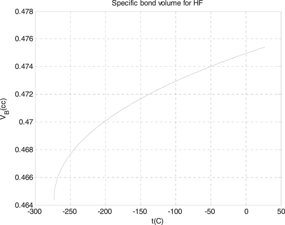
Figure 1. The specific bond volume of Morse potential for the hydrogen fluoride molecule.
Download figure:
Standard image High-resolution image
Figure 2. The specific bond volume of Morse potential for the hydrogen chloride molecule.
Download figure:
Standard image High-resolution imageThis thing of the differences is resulted from two things, the first one returns to the differences of the electronegativity between the two molecules, and the other returns to the volume of each molecule itself. We used the formula which we derived for the specific volume of the Morse potential for additional simple diatomic molecules, which are the hydrogen and nitrogen molecules. We plotted the results for these two molecules in figure 3 for the hydrogen molecules, with the depth of the well 4.7446 eV, and in figure 4 for nitrogen molecules, with the depth of the well 4.6618 eV.
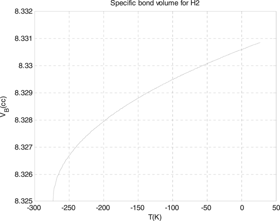
Figure 3. The specific bond volume of Morse potential for the hydrogen molecule.
Download figure:
Standard image High-resolution image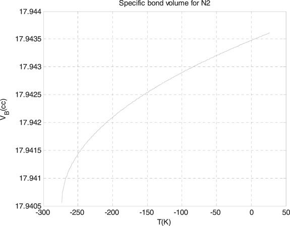
Figure 4. The specific bond volume of Morse potential for the hydrogen molecule.
Download figure:
Standard image High-resolution imageAs we see from figures 3 and 4, the specific bond volume of Morse potential for the hydrogen molecule is smaller than of the specific bond volume of Morse potential for the nitrogen molecule. Finally, we used the formula which we found for the specific bond volume of Morse potential for the slab–slider system [36] which is an important in the friction studies where the materials for the slider can be hard materials or soft materials. The slab–slider systems, generally, are composed of two different materials, one soft which is for the slab and the slider, and hard which is for the slider only. In table 1, we calculated the specific bond volume of Morse potential for the slab case, where the table includes the specific bond volume of Morse potential of the slab for different temperatures.
Table 1. The specific bond volume of Morse potential for the slab case with different temperatures.
| t (C) | −73 | −63 | −53 | −43 | −33 | −23 | −13 | 27 |
|---|---|---|---|---|---|---|---|---|
| VB (cc) (slab) | 0.6508 | 0.6518 | 0.6529 | 0.6549 | 0.6559 | 0.6568 | 0.6578 | 0.6604 |
In table 2, in table 1, we calculated the specific bond volume of Morse potential for the slider case in the hard materials case and soft materials case, where the table includes the specific bond volume of Morse potential of the slider for different temperature.
Table 2. The specific bond volume of Morse potential for the slider case in two cases hard materials slider and soft materials slider with different temperatures.
| t (C) | −73 | −63 | −53 | −43 | −33 | −23 | −13 | 27 |
|---|---|---|---|---|---|---|---|---|
| VB (cc) (hard) | 0.6051 | 0.6052 | 0.6053 | 0.6053 | 0.6054 | 0.6055 | 0.6055 | 0.6057 |
| VB (cc) (soft-materials) | 0.6508 | 0.6518 | 0.6529 | 0.6549 | 0.6559 | 0.6568 | 0.6578 | 0.6604 |
As we see from the two table, the changes of the hard materials specific bond volume of Morse potential is slower than the changes of the soft materials specific bond volume of Morse potential. Furthermore, we discussed the relation between the specific bond volume of Morse potential with temperature using the formula which we derived for the specific bond volume, for different values of the depth of the Morse potential well and for different values of the diameter of the particles of the system. The results of the specific bond of Mores potential versus temperature are plotted in figure 5(a) for four values of the depth of the Morse potential well, 0.01 eV (black curve—the highest curve), 0.1 eV (green curve), eV (red curve), and 10 eV (cyan curve—the lowest curve), and the results of the specific bond of Mores potential versus temperature are plotted in figure 5(b) for three values of the diameter of the particles, 0.1 nm (black curve—the lowest curve), 0.3 nm (green curve), and 0.5 nm (red curve—the highest curve).

Figure 5. The specific bond volume of Morse potential versus temperature for: (a) different values of the Morse potential well depth, (b) different values of the diameter of particles.
Download figure:
Standard image High-resolution imageAs it is shown in figure 5(a), the specific bond volume increases with temperature for all values of the depth of Morse potential and the greatest value of the specific bond volume returns to the smallest value of the depth of Morse potential well, which is 0.1 eV. Also, from the same figure, we see that the specific bond volume of Morse potential decreases when the depth of Morse potential well increases. Besides, we see from figure 5(b) that the specific bond volume of Morse potential increases with temperature for all values of the diameter of particles in the systems, and the largest value returns to the largest value of the diameter, which is 0.1 nm. In addition, we see from the figure that the specific bond volume of Morse potential increases when the diameter of particles composing the system increases. Also, we discussed the relation between the specific bond volume of Morse potential and the depth of Morse potential well and the results are plotted in figure 6 for three different temperature: −173 C (black curve—the lowest curve), zero Celsius degree (green curve), and 77 C (red curve—the highest curve).
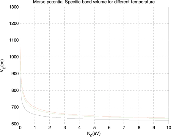
Figure 6. The specific bond volume of Morse potential versus the depth of Morse well for three different temperature.
Download figure:
Standard image High-resolution imageAs it can be seen from the figure 6, the specific bond volume of Morse potential decreases when the depth of Morse well increases for different values of temperatures, and after a specific value of the depth of the well, the specific bond volume of Morse potential decreases slowly. In addition, we see from the same figure that the largest value of the specific bond volume of Morse potential returns to the highest temperature. Finally, we discussed the relation between the specific bond volume of Morse potential and the molar volume of the system for three different temperature, we plotted the results in figure 7, where the black curve (the lowest curve) is for −173 C, the red curve is for 77 C (the highest curve), and the green one is for zero Celsius degree. As it can be seen from the last figure, the specific bond volume of Morse potential increases linearly with the molar volume of the system for the three values of temperatures.

Figure 7. The specific bond volume of Morse potential versus the molar volume for three different temperature.
Download figure:
Standard image High-resolution image
4. Conclusions
In this work, we derived an analytical formula of specific bond volume of Morse potential based on the theory of the integral equation in the statistical mechanics, where we found this bond volume based on the boundary conditions of the RDF, based on the solution of the OZE of the Morse potential for low density. We found that the specific bond volume of Morse potential has temperature dependence via logarithmic function and square root function. Also, we found that the specific bond volume of Morse potential is proportional to the molar volume of the system. We applied the derived formula for discussing the relation between the specific bond volume of Morse potential and temperature, we concluded that the specific bond volume, generally, increases with temperature increasing for different values of the depth of Morse potential well. Also, we applied the formula for discussing the relation between the specific bond volume of Morse potential and the depth of Morse potential well, we concluded that the relation between the specific bond volume of Morse potential decreases with increasing the depth of the well for a specific temperature. Also, we applied the derived formula for discussing the relation between the specific bond volume of Morse potential and the molar volume of the system, and we concluded that the specific bond volume of Morse potential increases via linear function with the molar volume of the system.
Besides, for discussing actual compounds, we applied the formula in case of four diatomic molecules, the first is the hydrogen chloride molecule, and the others are the hydrogen fluoride molecule, nitrogen molecule, and hydrogen molecule, we found that specific bond volume of Morse potential increasing with the absolute temperature for the four molecules. Also, we found that the specific bond volume of Morse potential for the hydrogen chloride is greater than of the specific bond volume of Morse potential for the hydrogen fluoride for the full range of the absolute temperature. Besides, we used the formula of the specific bond volume of Morse potential for calculating specific bond volume of Morse potential of the slab–slider system which is important system in the study of friction, where we applied the formula for two cases: hard and soft materials. We concluded that the specific bond volume of Morse potential of the hard materials changes is slower than the specific bond volume of Morse potential of the soft materials.
We believe that the formula for the specific bond volume of Morse potential which we derived in this study is general and can be applied to a wide spectrum of materials.
Conflict of interest
No.
Data availability statement
All data that support the findings of this study are included within the article (and any supplementary files).