

Abstract
This topical review presents an overview of the recent experimental and theoretical attempts on designing magnonic crystals for operation at different frequencies. The focus is put on the microscopic physical mechanisms involved in the formation of the magnonic band structure, allowed as well as forbidden magnon states in various systems, including ultrathin films, multilayers and artificial magnetic structures. The essential criteria for the formation of magnonic bandgaps in different frequency regimes are explained in connection with the magnon dynamics in such structures. The possibility of designing small-size magnonic crystals for operation at ultrahigh frequencies (terahertz and sub-terahertz regime) is discussed. Recently discovered magnonic crystals based on topological defects and using periodic Dzyaloshinskii–Moriya interaction, are outlined. Different types of magnonic crystals, capable of operation at different frequency regimes, are put within a rather unified picture.
Export citation and abstract BibTeX RIS
1. Introduction
1.1. The concept of magnetic excitations
In the recent years the study of spin waves or their quantised quasi-particles, magnons, in low-dimensional magnetic structures has become one of the most intriguing topics in condensed-matter physics. Investigation of magnons in magnetic materials has a long-standing prehistory in magnetism [1, 2]. Introducing the concept of magnons was essential to understand the physical origin of several observed phenomena in magnetic materials e.g., magnetic ordering at a finite temperature, magnetisation reversal process, electrical and heat conductivity, current induced magnetisation reversal and electron- as well as spin-dynamics [3, 4]. Figure 1 illustrates the importance of magnons in the fundamental understanding of different phenomena in solids.
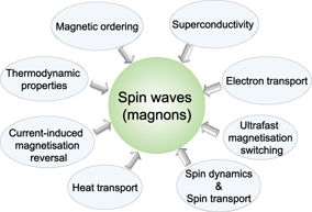
Figure 1. Illustration of the importance of magnons in fundamental understanding of different collective phenomena observed in condensed-matter physics.
Download figure:
Standard image High-resolution imageAfter the development of advanced fabrication methods of low-dimensional magnetic materials this field has entered a new level [5–9]. New magnon related phenomena such as magnon confinement, interference and localisation have been observed in low-dimensional magnets e.g., in ultrathin films and magnetic nanoelements [10, 11]. Discovery of these new phenomena has not only led to a much better fundamental understanding of magnetic nanostructures, it has led to the creation of a new research direction i.e., magnonics [12–19]. Within this research field one aims on utilising these newly discovered effects for practical applications in new generation of devices based on magnons [14, 17, 20, 21]. Recent advances in growth and nanofabrication techniques have now allowed the precise tailoring of the properties of magnons for such applications, making a large step towards realisation of nanoscale magnon-based devices.
1.2. The concept of magnonics
The concept of magnonics was primarily suggested to overcome the challenges in electronics. One of the main challenges in electronics has been the ohmic losses during the device operation. Such losses drastically reduce the efficiency of the devices, in terms of both energy and operation characteristics [13, 14, 17, 21]. The implementation of wave-based architectures was therefore suggested to be an alternative approach for performing non-volatile logic operations in a highly efficient manner. The idea was first suggested for photons, as quantum waves. It turned out that the use of magnons, as the representative quantum waves of magnetic excitations, shall have several additional advantages. First, the strong nonlinear effects of magnons would allow for designing more efficient and even multifunctional devices [20, 22–24]. Second, magnons can effectively be influenced by external stimuli such as electrical currents [25], magnetic [26] and electric [27–33] fields. Third, the magnon dispersion relation covers a rather wide range of frequencies starting from some megahertz (MHz) up to several tens of terahertz (THz). This would allow for a large choice of operation frequency of the devices. Likewise, the wavelength of magnons spans over a rather large range, from millimeters down to atomic scales (angstroms). Hence, realisation of a magnonic device with dimensions of a few nanometers and capable of operation within terahertz frequencies is, in principle, feasible.
1.3. The concept of magnonic crystals
A magnon-based device requires in the first step a platform on which different magnon modes can be excited [13, 14]. Such platforms should also allow for the manipulation of the magnon dispersion relation in a desired way. For that the concept of magnonic crystals (MCs) has been brought into discussion [34–38]. MCs are the analogues of photonic crystals (PCs), which have been used for the manipulation of photons [39]. In a similar manner MCs can be realised in order to manipulate the magnons. Such a crystal is usually created by periodic modulations in its magnetic properties. Periodic modulations in magnetic properties can be achieved using different approaches. For example, a magnetic structure containing periodic elements can be fabricated using standard nanofabrication (nanopatterning) techniques [5–7] or by other methods such as protein encapsulation [40] or growing on nanostructured templates [41]. Periodic modulations of the magnetic properties may be achieved by periodic modification of the structure of a magnetic medium (typically a thin magnetic film) by different means e.g., chemical etching [42, 43], laser processing [44, 45], ion implantation [46–48], interfacing the medium with other periodic magnetic or nonmagnetic nanoelements [49, 50], etc. In addition to these methods, periodic modulations of the magnetic properties may also be realised by changing the intrinsic properties without any modification of the sample structure. This can be achieved by periodic variation of local temperature [51], local internal magnetic field [52, 53], local magnetic state [7] or local spin texture [54].
Generally, MCs hold promise for miniaturisation down to nano-scales, since they can be designed in much smaller sizes compared to PCs. Since one of the goals is to integrate these structures in the existing electronic/spintronic technology and go even beyond that, one would require to make the size of the devices small (at least comparable to the size of the state-of-the-art electronic/spintronic devices). In the next step one aims on the miniaturisation of the devices, which would allow for more operations per chip area. One has to bare in mind that unlike the dispersion relation of photons, the one of magnons is anisotropic and can largely be tuned using an applied DC magnetic field. Furthermore, depending on the type of magnons excited in the system one may deal with different type of interactions e.g., dipolar or exchange interaction. These facts lead to characteristic and distinct differences between PCs and MCs.
This topical review is organised as following. In section 2 we provide the basic concepts needed to follow the topic. In sections 2.1 and 2.2 we briefly introduce the magnon dynamics in thin magnetic films and nanostructures. All types of magnons will be discussed. Section 2.3 is dedicated to the theoretical formalism used to describe the magnon band structure of MCs. The concept of magnon lifetime is briefly discussed in section 2.4. In section 3 different approaches used to realise MCs for operation in gigahertz and terahertz frequency regimes are discussed. We start with one and two dimensional MCs with magnon bands in gigahertz frequencies in section 3.1. We then extend the discussion to MCs for operation in terahertz regime in section 3.2. Other types of MCs are discussed in section 3.3. An overview on the possible applications of MCs, the possibility of designing reconfigurable devices, major challenges and possible solutions is presented in section 4. Section 5 provides a summary of the achievements and a perspective for the future works.
2. Magnonic band structure: From ultrathin films to magnonic crystals
2.1. Magnons in magnetic thin films and nanostructures
2.1.1. Uniform precession
When a spin system is driven out of equilibrium by a small perturbation, the most straightforward dynamics is the uniform precession, where all spins are equally canted and precess in phase. This uniform precession is referred to as ferromagnetic resonance (FMR) mode. In order to derive the equations for the FMR mode of a thin ferromagnetic film one may start with the Landau–Lifshitz–Gilbert (LLG) equation of motion

where M represents the magnetisation, Heff is the effective field, which consists of external as well as internal fields, γ is the gyro-magnetic ratio given by gμB/ℏ where g is the g-factor. α denotes the dimensionless damping parameter. Under some circumstances one can find analytical solutions describing the dynamics. Based on the FMR theory one can derive analytical expressions for the dispersion relation of the FMR mode (for details see [55]). Another approach is the one developed by Smit and Beljers [56], which is based on the consideration of the free energy of the system. Note that the FMR mode refers to the uniform precession of all spins and describes the magnons with the wavevector q = 0. Hence the dispersion relation in this case is usually referred to the dependency of the FMR frequency on the applied magnetic field. Using the first approach and after calculating the real and imaginary parts of the magnetic susceptibility, one can show that the imaginary part of the susceptibility, has the form of a Lorentzian function, which has its maximum at the FMR frequency.
Considering the coordinate system depicted in figure 2(a) for a thin film made of a single crystalline material ordered in a cubic structure [for example body-centered cubic (bcc) Fe] and considering only a uniaxial out-of-plane K2⊥ and a cubic K4 anisotropy the resonance frequency for the field applied along different directions will then be given by


Figure 2. (a) Illustration of the coordinate system for calculating the dispersion relation of the uniform precession in a magnetic thin film in the form of an infinitely large plate with the thickness d. (b) The dependency of the FMR frequency on the applied magnetic field calculated for an Fe film with μ0Meff = 2.14 T, the cubic anisotropy field of 2K4/M = 55 mT and the g-factor of g = 2.09. The blue (red) curve represents the calculation for the applied magnetic field in the film plane along the [100]–([110]) direction. The gray curves represent the calculations for intermediate directions between these two main symmetry axes.
Download figure:
Standard image High-resolution imageHere  denotes the effective out-of-plane anisotropy field (for details see for example [57, 58]). One should note that equations (2)–(4) are only valid for the saturated condition, i.e., H is strong enough to align all magnetic moments parallel to its direction. In an FMR experiment, however, for specific anisotropy values and directions of the external magnetic field the resonance conditions can also be fulfilled when M is not parallel to H. This causes an additional signal at smaller fields with lower intensity (unsaturated mode), when the FMR spectra are recorded at a fixed frequency and the external magnetic field is swept. Such unsaturated resonance modes have been observed in several experiments on Fe films [58–60]. In order to find the dispersion relation (frequency versus field) for the unsaturated mode numerical calculations are required.
In figure 2(b) the dispersion relation of the FMR mode (the dependency of the FMR frequency on the applied magnetic field) calculated for an Fe film with μ0Meff = 2.14 T, the cubic anisotropy field of 2K4/M = 55 mT and the g-factor of g = 2.09 is presented. The blue (red) curve represents the calculation for the applied magnetic field in the film plane along the [100]- ([110]) direction. The gray curves represent the calculations for intermediate directions between these two main symmetry axes. It is apparent that the dispersion relation even for the FMR mode is highly anisotropic in a magnetic film. This could also simply be observed by comparing equations (2)–(4). Another important consideration is that in the above mentioned formalism the confinement in the direction perpendicular to the film is neglected. This is a very good assumption for the limit of ultrathin films. Such an effect can simply be considered by adding an additional term into equation (2)

Here A represents the exchange stiffness constant and qz denotes the magnon wavevector in the direction perpendicular to the film. Since along this direction the film possess a certain thickness, qz takes only discrete values given by nπ/d, where n is an integer number. This implies that the thinner the film the larger the frequency associated with these modes. Such modes are traditionally called spin wave resonances and have been observed in FMR experiments performed on relatively thick films [61]. In the experiments only the odd modes could be observed. This was then explained by Kittel [62]. He showed that due to the boundary conditions, the modes with even numbers are not allowed to be excited (because the spins are assumed to be pinned at the boundaries of the sample, as a consequence of the surface magnetic anisotropy). Note that the uniform FMR mode is the one with n = 0. In equation (5) if one sets n to zero, one would obtain the same expression given by equation (2) i.e., the uniform FMR mode. The uniform FMR mode does not depend directly on the film thickness (it may indirectly depend on the thickness via thickness dependence of magnetic anisotropy and magnetisation).
Likewise one may introduce lateral confinements in the structure. In such a case it is important to consider the fact that the demagnetising factors need to be taken into account (in the above discussions we have assumed that the lateral dimensions are far larger than the film thickness). Furthermore, depending on the length-scales involved in the lateral confinement additional energy terms can come into play. For a simplified case with the field applied along the easy axis of the cubic anisotropy the dispersion relation will be given by
where, Nx, Ny and Nz represent the demagnetising factors along the x, y and z directions, respectively (see the coordinate system depicted in figure 2(a)) [63].
Geometrically confined ferromagnetic objects prepared by patterning the ferromagnetic structures exhibit nonuniformities. Such nonuniformities might be due to different reasons e.g., the static magnetic configuration of the object, the dynamic demagnetising fields, or even a deliberate design of magnetic inhomogeneities. As a consequence the local FMR frequency and the local dynamic susceptibility at different parts of the object will be different. This has been demonstrated in reference [64], where a methodology to efficiently calculate the local FMR frequencies is developed.
So far we have limited our discussion to the FMR mode in the limit of q → 0, where all the magnetic moments precess in phase, resulting an infinite wavelength of the magnon. In the next step we aim to consider magnons with q ≠ 0. Depending on the wavelength, the magnetic interaction dominating the magnons energy will be different. For the long wavelength excitations the dominating magnetic interactions are dipolar interactions. Hence these magnon modes are usually referred to as dipolar magnons. In the case of short wavelength magnons (wavelengths comparable to the interatomic distances) the relevant magnetic interaction is the magnetic exchange interaction. Consequently these magnons are referred to as exchange magnons. Magnons in the intermediate regime have both characters and are referred to as dipolar-exchange magnons. We shall briefly discuss different types of magnons in the following sections.
2.1.2. Dipolar magnons
The characteristics of dipolar or magnetostatic magnons have been introduced long ago [65]. Due to the anisotropic nature of the dipolar interaction the dispersion relation of this type of magnons depends strongly on the direction of the applied magnetic field and the shape of the sample. In the case of thin magnetic films one would expect three characteristic modes [55].
- The so-called magnetostatic surface wave (MSSW) refers to a magnon mode excited in a geometry in which q and H lie in the film plane but orthogonal to each other.
- The so-called magnetostatic backward volume wave (MSBVW) refers the case in which q and H are parallel and both lie in the film plane.
- Finally, the mode excited with q in the plane and H applied normal to the plane is called magnetostatic forward volume wave (MSFVW).
An illustration of the dispersion relation of all dipolar modes excited in a thin ferromagnetic film is presented in figure 3. The MSSW mode or the Damon–Eshbach (DE) mode shows a positive dispersion starting from the uniform FMR mode (Kittel mode) at q = 0. This mode is further characterised by the localisation of the magnons in the vicinity of the top and bottom surfaces of the film. In addition, this mode shows a nonreciprocal behaviour. The nonreciprocity of this mode implies that the magnons associated with this mode are differently localised at the top and bottom interfaces, depending on their propagation direction. This means that magnons with positive or negative sign of q travel either in the top or in the bottom layer. In other words the counter-propagating magnons propagate via the top or bottom part of the sample.

Figure 3. Calculated dipolar magnon dispersion relation for an Fe film with a thickness of 14 nm (≃100 atomic layers) according to equations (7)–(9). The parameters used for the calculation were as follows. The effective out-of-plane anisotropy field was μ0Meff = 2.14 T, the cubic anisotropy field was 2K4/M = 55 mT and the g-factor was g = 2.09. While the green curve denotes the magnetostatic surface waves, the blue and red curves represent the magnetostatic forward and backward volume modes, respectively. In the case of MSSW and MSBVW the magnetic field was applied in the film plane along the [100] direction. In the case of MSFVW the magnetic field was applied along the [001] direction.
Download figure:
Standard image High-resolution imageThe dispersion relation of the MSSW mode has the from of
The dispersion relation of the MSBVW mode is given by
In the equations above q∥ represent the parallel momentum i.e., the component of the wavevector which lies the film plane. The MSBVW mode exhibits a negative group velocity. Another characteristic of this mode is that, in contrast to the MSSW mode, its amplitude is distributed throughout the volume part of the film.
The dispersion relation of the MSFVW mode is given by
Similar to MSSW, this mode also possesses a positive group velocity. Unlike MSSW the amplitude of this mode is distributed over the volume part of the film. The dispersion relation of this mode is isotropic in the film plane meaning that it does not depend on the direction of q∥.
2.1.3. Exchange magnons
These magnons are governed by the magnetic exchange interaction, usually referred to as Heisenberg exchange. Since this interaction is rather short-range one has to use a microscopic picture in order to describe the exchange magnons. The Heisenberg Hamiltonian describing the interaction between magnetic moments siting on lattice site i and j reads as

where Jij denotes the symmetric Heisenberg exchange constant and the unit vectors êi and êj represent the direction of the magnetic moments at the atomic sites i and j, respectively. For simplicity we set the amplitude of spin to unity S = 1. In this picture magnons are the low-energy excitations associated with small-amplitude precessions of moments around the main magnetisation direction. In the case of bulk single-element ferromagnets expanded in the three dimensional space one expects to observe a single magnon band [55]. However, in magnetic films composed of several atomic layers one can show that, in principle, m magnon modes are expected to be observed [66–68]. The dispersion relation of these modes can be calculated by starting from equation (10) and finding the solution of the following matrix equation
where R = Ri − Rj with Ri and Rj being the position vector of sites i and j, respectively. Aj (j = 1 to m) represent the amplitude of the magnons. Equation (11) indicates that for a magnetic film composed of m atomic layers one should observe m different magnon modes. There will be two magnon modes, which are lower in frequency with respect to the others. Those modes are formed due to the lower coordination number of magnetic moments in the top and bottom layers of the film. At q = 0 these two modes are separated by ω(q = 2π/md) in frequency, where d represents the interatomic distance. We assume that the interatomic distances in all directions are the same. In case that the same values of exchange constants are considered at the top and bottom layers, these two modes will degenerate in frequency at high wavevectors, close to the zone boundary. It is apparent from equation (11) that this quantity depends on the exchange constants as well. For a given magnon mode Aj varies from one layer to another. Therefore this quantity might be considered as the contribution of each layer to that particular mode. For example the two lowest-frequency magnon modes have the largest amplitude of the eigenvectors in the top and bottom layers. This means that these modes are localised at these two layers. If these two layers are magnetically identical it is not possible to distinguish between them. However, if the layers are magnetically different (the values of the exchange parameters or the amplitude of the moments in the layers are different) the degeneracy of these two low frequency modes will break and one can associate a mode to each layer. This is of particular importance and will be discussed further in section 2.3.2.
As an example we show in figure 4 the exchange-dominated magnons calculated based on a Heisenberg model for an Fe film composed of six atomic layers. The calculations are performed for a simplified case, where only the nearest and next nearest neighbours are taken into account. The assumption here is that the nearest neighbour exchange constant is Jn = 8.9 meV, the next nearest neighbour exchange constant is J2n = 0.6Jn and the higher order terms are zero (J3n = J4n = ... = 0). The calculations are performed for the first and second Brillouin zone (BZ). The characteristics of the exchange magnons are as follows. (i) The modes with low quantum number show a semiparabolic dispersion for the limit of small q∥. This means that the group velocity of such magnons, given by  , increases linearly with q∥ up to the zone boundary. This behaviour can be different for modes with a large quantum number. The fact that the film possess a translational symmetry in the plane is reflected in the fact that the dispersion relation is perfectly reproduced while going from the first to the second BZ. (ii) The frequency of these magnons exceeds quickly the terahertz regime.
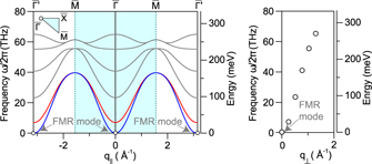
Figure 4. Calculated exchange magnon dispersion relation for an Fe film with a thickness of 6 atomic layers (≈0.9 nm) based on a Heisenberg model [equation (11)]. The exchange parameters used for the calculation were Jn = 8.9 meV and J2n = 0.6Jn. The dispersion along the main symmetry  –
– direction of the surface BZ (the [100] direction in real space) is shown in the left side and the one along the normal direction (the [001] direction) is shown in the right side. The calculations are performed over the first and second surface BZ. Inset illustrates the surface BZ.
Download figure:
Standard image High-resolution imageConventionally, the lowest frequency magnon mode, which satisfies the Goldstone criteria, is the so-called 'acoustic mode' (curve shown in blue colour in figure 4). The higher energy magnon modes are the so-called 'optical modes', which possess a finite energy at q∥ = 0, in analogy to the phonon modes in solids.
Note that the assumptions made above break in the limit of q∥ → 0. This is due to the fact that at this limit the other interactions become important and must be considered in the description of the magnon dispersion relation. This is why even the uniform FMR mode possesses a finite frequency (see figure 3).
It is important to notice that although the magnon modes shown in figure 4 are the result of quantum confinement in the direction perpendicular to the film, they exhibit a finite momentum in the film plane (finite q∥). This means that these magnons can propagate through the system with a certain group and phase velocity.
In a similar manner one can also calculate the eigenstates based on equation (11). The eigenstates would provide the profile of different magnon modes. An easier way to treat the mode profiles would be to just analyse the amplitude of the eigenstates. This would provide all the necessary information regarding the localisation of different modes. As discussed above the first two modes indicated by the blue and red colours are the modes mainly localised in the top and bottom surfaces. Since the spins sitting in these two layers possess less neighbours than those sitting in the volume part of the film, these two modes are lower in frequency, compared to the others. In the calculations shown in figure 4 all the layers are treated equally and hence the top and bottom layers are identical. This means that the amplitudes of the eigenvectors for magnons describing these two modes, given by equation (11), will be equal in the top and bottom layers. In the case of real systems (ferromagnetic film grown on a nonmagnetic substrate) the presence of the substrate breaks the degeneracy of these two modes and leads to the nonequivalent localisation of these modes in the top and bottom layer. Another consequence of the identical exchange parameters in these two layers is the degeneracy of the modes near and at the zone boundary ( -point).
The magnon momentum in the direction perpendicular to the layers is confined and takes only discrete values q⊥ = nπ/m, where m is the number of atomic layers and n is the mode number, being 0, 1, ..., m − 1 [see the right side of figure 4]. Note that here it is assumed that the spins are all exchange coupled. This, in turn, means that the spins are unpinned at the two interfaces. In a thin magnetic film with a finite thickness the magnons with quantised q⊥ = qz and zero parallel momentum, q∥ = 0, can be excited also in the gigahertz regime, when the film thickness is several tens of nanometers. These magnon modes are the spin wave resonances as described earlier in section 2.1.1. Their dispersion relation is given by equation (5). It has been demonstrated that due to the boundary conditions only the odd resonance modes can be observed in experiments (see for example [61] for details).
2.1.4. Dipolar-exchange magnons
The intermediate regime between the dipolar and exchange magnons is the so-called dipolar-exchange regime. Obviously, both the dipolar and exchange terms need to be considered in order to describe this regime. It has been shown that in the presence of the exchange field additional boundary conditions need to be considered. These boundary conditions are usually referred to as exchange boundary conditions, which imply that at the film boundaries the precession of moments depends on the surface anisotropy present in the system. Kalinikos and Slavin have derived a practical expression for the dispersion relation of dipole-exchange magnons in a thin ferromagnetic film subject to arbitrary exchange boundary conditions, when the magnetic field is applied in the film plane [69]
The wavevector q can be decomposed to the parallel and perpendicular components. Since for a thin film the perpendicular component is quantised one can therefore write  . Here again q∥ denotes the in-plane component of the magnon wavevector. Tnn describes the matrix element of the dipole-dipole interaction and in a general form is given by
Here φq denotes the angle between q and M. Under the assumption that the surface moments are fully unpinned and if the magnetisation is fully uniform across the thickness, Pnn can be simplified to

A graphical visualisation of the dipolar-exchange magnons in an Fe film is presented in figure 5. It is apparent that confinement effects can drastically change the dispersion relation of these magnons. The most simplest picture is that the wavevector will no longer be a continuous quantity and will only choose discrete values. In the next section we will discuss how the confinement effects change the magnon dispersion.
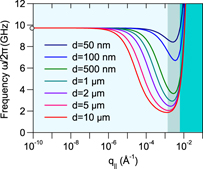
Figure 5. Calculated dipolar-exchange magnon dispersion relation for Fe films of different thicknesses according to equations (12)–(14). q was assumed to be in the film plane and parallel to the magnetisation (q = q∥ and φq = 0). The parameters used for the calculation were as follows. The effective out-of-plane anisotropy field was μ0Meff = 2.14 T, the cubic anisotropy field was 2K4/M = 55 mT, the exchange stiffness A = 20.4 pJ m−1 and the g-factor was g = 2.09. In all cases the magnetic field was applied in the film plane along the [100] direction. Different regimes are shown by different colours. For q∥ < 10−3 Å−1 the magnons are determined by the dipolar interaction (light green). Magnons with q∥ > 10−2 Å−1 are determined by the exchange interaction (dark green). The intermediate regime is the dipolar-exchange regime.
Download figure:
Standard image High-resolution image2.2. Magnons in laterally confined ferromagnets
When an infinitely extended film is laterally confined in one or two dimensions in the form of stripes, rectangular or polygonal elements two more considerations are required. First, the demagnetising fields have to be taken into consideration (similar to the discussion related to equation (6) in section 2.1.1). Second, the lateral confinement may lead to the appearance of additional magnon modes due to several reasons (see the discussion below). The lateral confinement has therefore direct consequences on dipolar, dipolar-exchange and exchange magnons. In the following we consider all these types of magnons. Instead of deriving equations for the magnon dispersion relation we provide a qualitative explanation of the phenomena occurring as a result of the lateral confinement.
Generally, the number of magnon modes increases when reducing the dimension of the system [70–72] (even the FMR mode [73]). The properties of the new modes depend strongly on the geometry of the system, the length-scales involved, new effects associated with confinement (new boundary conditions [74, 75], dynamical pining, etc.), the direction of the static magnetisation and the orientation of the external magnetic field.
Let us now consider a ferromagnetic stripe for which the aspect ratio is small (p = w/l ≪ 1, where w represents the width of the element and l denotes its length). Now if the stripe is magnetised along the length, the most prominent result of lateral confinement is the quantisation of the in-plane wavevector along the width of the stripe [76, 77]. However, if the stripe is magnetised along its width, one has to consider the demagnetising effects. In such a case demagnetising effects are rather strong and lead to a reduction of the internal fields in the vicinity of the edges (see figure 6). This effect results in a potential well for the magnons, which then lead to modes localised near the edges of the stripe [78, 79]. These modes are sometimes referred to as edge modes. In rectangular platelets, both effects are present [80–82]. Considering the geometry shown in figure 6, if the external magnetic field is applied parallel to the y direction, the effects associated with demagnetising are fairly negligible. It has been shown that dynamic dipolar fields generated by the dynamical magnetisation in the vicinity of the edges are inhomogeneous. Such fields result in a phenomenon called dipolar pinning, which leads to the quantisation of magnons with the component of q along the width of the stripe i.e., qx. It has been shown, that the quantised frequencies of these magnon modes can be approximated by [83]
Here the integer number n' represent the quantisation of the qx in the width of the stripe. Once more we should emphasis that the assumption here is that p is very small.

Figure 6. Calculated internal magnetic fields across a ferromagnetic Fe stripe with the width of 500 μm (left). Calculated dipolar-exchange magnon dispersion relation for this stripe (right). The direction of q is specified in the left side (it is along the width of the stripe i.e., x direction). The stripe is magnetised along its width (x direction). The dispersion relation is calculated for different points as shown by different colours in the left graph. For the point shown by the green colour the dispersion relation exhibits a minimum at about qx = 0.0025 Å−1. A magnon excited at the edge region with zero field at the frequency of about 3 GHz propagates towards the centre of the stripe, adjusting its wavevector until reaching the extremum point at the green dot. The magnons is, therefore, reflected, leading to the formation of an edge mode. For simplicity in these illustrative calculations we neglect the cubic anisotropy.
Download figure:
Standard image High-resolution imageNow let us consider that the external magnetic field is applied along the width of the stripe (along the x direction). In such a case the demagnetising effects are very strong and lead to inhomogeneous internal fields across the stripe. Considering the geometrical parameters such inhomogeneous internal fields can be calculated. In figure 6 a plot of the internal fields across a stripe made of Fe is plotted, indicating its nonuniform profile. Now based on equation (12) one can calculate the dispersion relation of the modes formed in different locations in the stripe. A plot of the dispersion relation of the magnetostatic dipolar and dipolar-exchange magnons for three different points across the stripe is shown in figure 6. Now if the propagating magnon propagates from the edge of the stripe towards the centre its wavevector shall change continuously in order to satisfy the dispersion relation. The magnon will be reflected at the point where the internal magnetic field increases sufficiently so that no solution for the dispersion relation with real value of momentum exists. Hence, the magnon of this kind is localised in the vicinity of the edges of the stripe [10].
For the confinement in both directions i.e., in the case of a rectangular element, one needs to consider the effects mentioned above in both directions. In such a case the magnon dispersion relation will be modified twofold. The system may be treated by decomposing the components of magnons and the effects associated with the confinement in two directions. Since in this case it is rather difficult to calculate the demagnetising factors analytically and the equations describing the dispersion relations become more complex, a better approach would be to use the numerical methods to calculate the dispersion relation.
It is worth mentioning that, in principle, nonuniform demagnetising fields in a confined magnetic element can lead to the emission of magnons. This has been discussed in references [84, 85]. It has been suggested that the effect may be used to excite magnons of different frequencies. We will come back to this point later in section 4.3.2.
2.3. Magnons in magnonic crystals
As discussed above the magnon dynamics depends on the geometrical shape of the magnetic element. Hence, it is, in principle, possible to design magnetic structures, which can act as platform for magnons. Moreover, by tuning the magnetic properties of these platforms one would be able to change the characteristics of magnons in such structures. One of the elegant ways to design such platforms is taking advantage of lateral confinements and design periodic structures, which can be used as MCs. Such an idea can be realised in the same way as it is done for PCs.
The essential considerations required to understand the magnons in MCs are those introduced in sections 2.1 and 2.2 for the magnons in reduced dimensions. In order to describe the magnon dynamics in MCs in the following we first categorise them in two classes; MCs for magnons with long wavelength (gigahertz magnons) and MCs for magnons with short wavelength (terahertz magnons).
2.3.1. Magnonic crystals for gigahertz magnons
The magnon dispersion relation in MCs with periodic modulations in the magnetic properties can be understood in the same way as the formation of the electronic bands in a solid as a result of the periodic arrangement of atoms. The magnon dispersion relation is therefore commonly called the magnonic band structure. Such a band structure can be efficiently calculated using the so-called plane wave method, which is analogous to the Bloch description for electronic states in solids [72, 86–91]. In the following we just briefly introduce this approach. Another approach is based on the Walker's equation [92]. We do not, however, discuss it in the present topical review.
Let us consider a magnetic thin film with a thickness much smaller than the lateral extension. Now if one introduces lateral variation of magnetic properties in one or two dimensions an MC may be realised. This general idea is schematically illustrated in figure 7. Note that for simplicity we only consider MCs of ultrathin films. One may also think of periodicity in the third direction. The physics of those systems would be somewhat similar. We do not treat those structures in the present topical review.
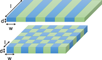
Figure 7. Illustration of the idea of thin film 1D and 2D MCs by introducing lateral variation of magnetic properties in one and two dimensions. The periodic variation of magnetic properties may be realised either by modulation of the intrinsic magnetic properties (without modulation of the structure) or by modulation of the structure. The magnetic properties, which may be periodically modulated are magnetisation, local internal fields and magnetic anisotropy. Such modulations may be realised by several means e.g., variation in the thickness, materials composition, chemical properties, local strain, temperature, magnetic or electric fields. The properties of such MCs may be tuned by variation in width w, length l or the thickness d of each element as well as the geometrical factors of the periodic structure e.g., lattice structure or lattice constant.
Download figure:
Standard image High-resolution imageThe periodic variation of magnetic properties may be realised either by modulation of the intrinsic magnetic properties (without modulation of the structure) or by modulation of the structure. According to equations (3)–(9) and (12) the magnetic properties, which may be periodically modulated are magnetisation, local internal fields and magnetic anisotropy. Such modulations may be realised by several means e.g., variation in the thickness [93–96], materials composition [49, 50, 97–103], chemical properties [104, 105] or local strain, temperature, magnetic states, spin texture and magnetic field [51–54]. The structure might be single or bi-component [89, 106–113]. The basic idea behind is essentially the same.
Considering a periodic modulation of the saturation magnetisation and solving the LLG equation [equation (1)] one can calculate the magnonic band structure. In such a case the Heff includes the external applied field H, the anisotropy fields Hani, the exchange field Hex and finally the magnetostatic field Hms caused by magneostatic interactions. If one assumes that the magnons having a long wavelength have a uniform profile in the z direction, perpendicular to the periodic structure, one can simplify the picture for a 2D array of magnetic elements. Now if one assumes the form of  and
and  ) for the dynamical magnetisation and the magnetic field, respectively, one can simplify the solution of the LLG equation to the following coupled equations

Here Ω represents the normalised frequency and is given by Ω = ω/γμ0H. Considering the limit of the uniform mode, one can write the component of the dynamical magnetisation as

In order to find the solution now one has to apply the boundary conditions

Inserting equations (17) and (18) into equation (16), one can obtain an equation for the dispersion relation.
Now one should consider the periodic modulation of M in the structure. This can be done in the same way as it is done for electrons in a solid. The magnetisation can be written in terms of its Fourier component.

where ![$\boldsymbol{G}={\left[{G}_{n},\;{G}_{m}\right]}^{\mathrm{T}}={\left[\frac{2\pi n}{a},\frac{2\pi m}{b}\right]}^{\mathrm{T}}$](https://content.cld.iop.org/journals/0953-8984/32/36/363001/revision2/cmab88f2ieqn9.gif) represents a two-dimensional vector of the reciprocal lattice with periodicity along the two main directions x and y, given by the lattice constants a and b, respectively. The Fourier component M(G) is the key quantity defining the properties of the MC, as it can define the geometry (and the symmetry) of the system. Note that in this simple formalism modulations in other material constants are not taken into consideration.
represents a two-dimensional vector of the reciprocal lattice with periodicity along the two main directions x and y, given by the lattice constants a and b, respectively. The Fourier component M(G) is the key quantity defining the properties of the MC, as it can define the geometry (and the symmetry) of the system. Note that in this simple formalism modulations in other material constants are not taken into consideration.
The solutions of equation (16) in general form are Bloch waves

Inserting equation (20) in equation (16) the dynamic magnetic field components can be calculated. Equations (19), (20) and (16) provide a system of equations in the case of finite number of G, which can be summarised in the form of

where, ![${\boldsymbol{m}}_{\boldsymbol{q}}^{j}={\left[{m}_{y,\boldsymbol{q}}^{j}\left({\boldsymbol{G}}_{1}\right),\dots ,{m}_{y,\boldsymbol{q}}^{j}\left({\boldsymbol{G}}_{N}\right),{m}_{z,\boldsymbol{q}}^{j}\left({\boldsymbol{G}}_{1}\right),\dots ,{m}_{z,\boldsymbol{q}}^{j}\left({\boldsymbol{G}}_{N}\right)\right]}^{T}$](https://content.cld.iop.org/journals/0953-8984/32/36/363001/revision2/cmab88f2ieqn10.gif) . The eigenvalues Ωi = ωi/γμ0H would provide the dispersion relation of the modes associated with the respective periodic structure. In addition to this the eigenvectors
. The eigenvalues Ωi = ωi/γμ0H would provide the dispersion relation of the modes associated with the respective periodic structure. In addition to this the eigenvectors  would provide the mode profile. The calculation of the eigenvectors is of particular importance when one aims to see how different magnon modes are formed and where these modes are mainly localised. The norm of the amplitude of the eigenvectors would results in the degree of localisation of each mode in different parts of the structure. The 2N × 2N-matrix
  has a block-diagonal form

where  and the terms of the off-diagonal sub-matrices are given by
In the above equation the locally varying static demagnetising field Hdem has been taken into account by including a Bloch type of function of this field in the form of

The exact form of Hdem(r) can be obtained either by analytical expressions of the demagnetising factor or more practically by micromagnetic simulations. The presence of Hdem(r) can, in principle, change the boundary conditions and hence has a direct consequence on the magnonic band structure of MCs. In order to obtain the dispersion relation one needs to accurately calculate the periodic potential of the system. For that one needs to consider many reciprocal lattice vectors. This may violate the assumption that the magnon wavelength is much larger than the thickness of the sample. This means that while comparing the results of such calculations to those of real systems, measured experimentally, the lowest order branches should show a good quantitative agreement.
Note that for simplicity in the above formalism modulations in the exchange field has not been taken into account. Such effects can be included by adding the following expression into the effective field in the LLG equation.

where the exchange length lex(r) is given by  . Consequently one needs to define the Fourier component of the exchange length as

In order to better understand the effect of the lateral confinement and the periodicity of the structure on the magnonic band structure let us first consider the so-called empty lattice model (ELM). Based on the Bloch theorem in solids the presence of the translational symmetry in a crystal introduces the periodicity of the dispersion relation. The period of this periodicity is given by G. For an illustration this effect is calculated for the MSBVW mode excited in a permalloy film with a thickness of d = 20 nm. The lattice parameter of the artificial square lattice was a = 314 nm. The results are shown in the right side of figure 8. For a clear representation we use the so-called extended zone scheme. It is apparent from figure 8 that the single mode of the extended thin film, as expected from equations (8) and (12), is now changed to several magnon branches, as a result of back-folding. The single-band system is now developed into a multi-magnon band system. The magnonic band structure exhibits several degenerate magnon states at the zone centre. In order to shed light on the origin of these states one may analyse the magnon eigenvectors. The eigenvectors provide the mode profiles of different magnon modes. The calculated mode profile of different crossing points at the zone centre are shown in the left side of figure 8, indicating that the degenerate magnon states at this high symmetry point are the result of the fact that these modes represent magnons which differ only in their phase by G. The qx value of these magnons is quantised and is given 2π/a, 4π/a, 6π/a, .... It is important to mention that the folding of the dispersion band within the ELM approximation is rather fictional. This is opposed to the case of real MCs.
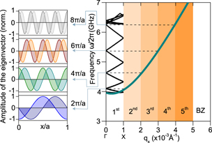
Figure 8. Calculated magnonic band structure in the ELM approximation for magnons in a structured permalloy film in the backward volume geometry. The dispersion relation is calculated in the extended zone scheme up to the fifth BZ. The thickness of the film was d = 20 nm and the artificial lattice was assumed to have a square form with the lattice constant of a = 314 nm. The eigenvectors of the degenerate points at the zone centre are shown in the left side. The qx value of these magnons is quantised and is given by 2π/a, 4π/a, 6π/a, .... The eigenvectors of magnons at these degenerate points differ only in their phase with one reciprocal lattice vector G.
Download figure:
Standard image High-resolution imageBased on the same arguments one can show that for the DE geometry in which the applied magnetic field and the wavevector are orthogonal to each other one would expect the appearance of additional magnon modes as a result of periodicity in the structure.
Using the formalism discussed above one may calculate the magnon band structure for an MC composed of ferromagnetic nano-elements embedded in a matrix made out of a different ferromagnetic material. A comparison between such results with those of ELM would provide useful information regarding the effect of the periodic potential on the magnonic band structure. An example of such analysis is provided in reference [89]. The magnon band structure for a system composed of Co nanodots embedded in a permalloy matrix as calculated by Krawczyk et al is shown in figure 9. The band structure calculations have been performed for a sample with a thickness of d = 20 nm, a lattice constant of a = b = 600 μm and a dot diameter 2R = 310 nm. Note that for this system the demagnetising factors can be calculated analytically [114, 115]. A magnetic field of μ0H = 20 mT, applied along one of the main symmetry axis in the plane has been assumed, as depicted in figure 9.
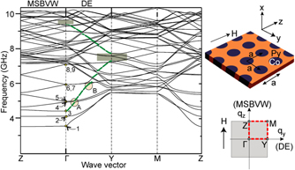
Figure 9. The magnonic band structure of an MC composed of Co nanodots embedded in a permalloy matrix. The calculations have been performed for both the DE and MSBVW geometries by Krawczyk et al [89]. The real space structure and the corresponding reciprocal space representation are shown in the right side. The green dashed curve indicates the DE mode in the first BZ. The hybridisation between the DE mode with the other magnon modes is highlighted by the capital letters A and B. The magnonic band splittings are marked with the shaded rectangular areas. Adopted from Krawczyk et al [89]. © IOP Publishing Ltd. All rights reserved.
Download figure:
Standard image High-resolution imageThe magnonic band structure exhibits several bands, even in the low-frequency part of the spectrum. However, the first order mode seems to appear at very low frequencies, even below the FMR frequency of the system. This has its origin in the fact that internal fields along this particular direction are small. The effect is very similar to the one discussed for the magnetic stripes in section 2.2 and in figure 6. Owing to the presence of boundaries the internal field is not homogeneous, unlike the case of a continuous film. The field profile leads to the formation of periodic potentials, which confine the magnons. Since the magnons representing these modes propagate through the part of the structure with internal fields of lower magnitude, the frequency of these modes becomes lower, compared to a continuous film.
Another essential observation is that the degeneracy of the modes at the zone centre is lifted. This is due to the fact that the mode profile associated with each of these points has a different shape across the structure (these modes are differently distributed). Consequently, it is important to see where the maximum amplitude of these modes is located (on the dots or on the spaces between the dots). In other words nonuniform pattern of demagnetising fields across the structure leads to the fact that the modes do not degenerate at the zone centre. The splitting of the modes depend on the frequency. As a rule of thumb the higher the frequency of the modes the smaller the splitting.
Another important phenomenon which originates from the interaction of different magnon modes in an MC is the appearance of the so-called avoided-crossing regions in the magnon band structure. These regions which are shown by circles in figure 9 indicate the presence of interaction between different magnon modes. Since avoided-crossing takes place only for modes having the same symmetry, one should not expect it for all modes. This is a general phenomenon observed for quasi-particles in periodic potentials. Hence an analysis of the symmetry of the modes would account for the identification of the regions with avoided-crossing [116].
The final and the most important observation is the appearance of several band splittings in the band structure (shown by shaded area in figure 9). The origin of these splittings which can clearly be observed for the DE mode lies in the destructive interference of Bragg reflected magnons at the boundary of BZ [43, 117, 118]. The most intuitive picture of the Bragg mechanism is as follows. Consider a wave travelling through a one dimensional periodic medium. If the Bragg conditions are not fulfilled the wave can easily propagate through. However, if the Bragg conditions are fulfilled the wave will be reflected backwards. In such a case one would expect a constructive or distractive interference, depending on the phase relation between the waves. The interference leads to the formation of standing waves and the presence of band splittings in the dispersion relation at the high symmetry points. Such an effect is expected for magnons as well. The magnitude of such a band splitting depends on the materials parameter, the applied magnetic field and the geometry of the sample [119]. For some cases an analytical expression for the amplitude of the band splitting can be derived (see for example [114]).
The band splitting is the first step towards designing a system with a bandgap through the whole BZ. In order to open such a bandgap one should reduce the anisotropy of the DE and MSBVW modes. If the frequency of the DE mode at the boundary of the first BZ is smaller than the frequencies of MSBVW, one would expect a bandgap opening. Such conditions are never fulfilled in a square lattice. In references [120–124] the changes in the geometrical structure have been examined. However, no full magnonic gap could be observed for the studied structures. As a side remark, it is rather straightforward to imagine that since in the case of MSFVW the dispersion relation is isotropic one would be able to open full magnonic bandgaps [125].
2.3.2. Magnonic crystals for terahertz magnons
The above discussion was limited to the dipolar and dipolar-exchange magnons. Exploiting the pure exchange magnons would open new possibilities to take advantage of high group/phase velocity as well as high frequency of this type of magnons. Moreover, since these magnons are governed by the short range exchange interaction, they would allow one to design MCs on much smaller length-scales.
As discussed in section 2.1.3 the magnon band structure of the exchange-dominated magnons can be calculated based on equation (11). Since the magnetic exchange interaction is rather short range in a single-crystalline sample the periodicity in the magnetic energy is given by the atomic arrangement i.e, the periodicity of the lattice. Assuming that the magnetic exchange interaction is isotropic (this is the case for most of the cubic crystals) the dispersion relation is also isotropic along the equivalent symmetry directions. For an infinitely extended sample in three dimensional space the Heisenberg model predicts only a single magnon band. This is due to the fact that all the magnon bands of such a system degenerate in energy. If the idea is to break the degeneracy of these bands, one may introduce additional periodicity on the atomic scales, for instance by replacing every second magnetic atom with another type. Under the assumption that the Heisenberg exchange is not affected, this leads to the fact that the spins on different sublattices will have different magnitudes and hence the degeneracy of the magnon bands will be lifted. In other words the magnetic unit cell becomes bigger. The larger the number of atoms in the unit cell the larger the number of magnon bands. In the next step if the idea is to open bandgaps in the magnonic band structure one needs to satisfy the conditions that the maximum frequency of the lower band is always lower than the minimum frequency of the upper band. This condition may be satisfied by taking different strategies (see the discussion below).
In the case of ferrimagnetic materials, in which the magnitude of the spin sitting on different sublattices is different, it has been often observed that the system exhibits several branches for exchange magnons. However, the magnitude of magnetic moments and the exchange parameters describing the interaction of spins are somehow interconnected. Since both the magnitude of moments and the values of exchange parameters are intrinsic properties of the material, tuning them in a desired way is not an easy task. Moreover, ferrimagnets often exhibit a rather complex structure, which adds to the complication of the problem.
Another approach as has recently been proposed is using the synthetic layered structures made of atomically smooth ultrathin ferromagnetic layers [126]. In order to illustrate the idea let us first discuss how the magnonic band structure develops in a layered ferromagnet. For simplicity we consider a ferromagnet ordered in a face-centered cubic (fcc) structure. The choice of fcc structure is based on the fact that due to its symmetry the nearest neighbours exist in both the individual atomic plane as well as the neighbouring atomic planes. This is not the case for a bcc lattice and hence one would expect additional effects due to the change in the number of nearest neighbours. The calculated magnon dispersion relation for an atomic layer of such a structure, based on equation (10) and considering only the nearest neighbour interactions, is shown in figure 10(a). The system shows a single magnon band with the maximum frequencies at the zone boundary. Now if one adds an additional layer on top of this layer, due to the fact that magnons with a phase relation of π are also allowed to form in such a bilayer structure, one will observe an additional magnon band, as shown in figure 10(b). In the case of a film composed of three atomic layers one should observe three magnon modes [see figure 10(c)]. The first two modes exhibit a similar dispersion relation and are equally distributed in the top and bottom atomic layer. The third mode is the result of strong coupling of the middle layer to these two layers. The opened partial bandgap along the  –
– direction is a result of the complete 'magnetic unit cell'. The magnitude of the bandgap is determined by the minimum of the n = 2 magnon band and the maximum of the n = 1 magnon band. The minimum of the n = 2 magnon band is either at the
  -point or at the
  -point. The maximum of the n = 1 magnon is at the
  -point. The bandgap is therefore given by
 ![${{\Delta}}_{\bar{{\Gamma}}-\bar{\mathrm{X}}}^{\mathrm{O}\mathrm{M}\mathrm{B}\mathrm{G}}=\left(1/2\pi \right)\left[{\omega }_{n=2}\left(\overline{{\Gamma}}\;\mathrm{o}\mathrm{r}\;\overline{\mathrm{X}}\right)-{\omega }_{n=1}\left(\overline{\mathrm{X}}\right)\right]=8JS/h$](https://content.cld.iop.org/journals/0953-8984/32/36/363001/revision2/cmab88f2ieqn20.gif) . Since this gap in opened between the optical magnons it may be called optical magnon bandgap (OMBG).
. Since this gap in opened between the optical magnons it may be called optical magnon bandgap (OMBG).

Figure 10. Evolution of the magnonic band structure with the number of atomic layers. The calculated magnon band structure for one (a), two (b) and three [(c) and (d)] atomic layers of a ferromagnetic film ordered in the fcc(100) stacking. The corresponding surface BZ is depicted as the inset in (a). The atomic arrangements considered for the calculations are shown from both top and side views on top of each graph. In all calculations only the nearest neighbour interactions were taken into account. In the calculations shown in (a)–(c) the exchange interaction was assumed to be isotropic (J∥ = J⊥ = J). In (c) an OMBG is opened along the  –
– direction. The magnitude of the bandgap is given by
 ![${{\Delta}}_{\bar{{\Gamma}}-\bar{\mathrm{X}}}^{\mathrm{O}\mathrm{M}\mathrm{B}\mathrm{G}}=\left(1/2\pi \right)\left[{\omega }_{n=2}\left(\overline{{\Gamma}}\;\mathrm{o}\mathrm{r}\;\overline{\mathrm{X}}\right)-{\omega }_{n=1}\left(\overline{\mathrm{X}}\right)\right]=8JS/h$](https://content.cld.iop.org/journals/0953-8984/32/36/363001/revision2/cmab88f2ieqn23.gif) . In (d) the exchange interaction was assumed to be anisotropic (J∥ = J and J⊥ = 1.5J). A full OMBG is predicted in this case. The bandgap spans over the whole surface BZ and is given by
. In (d) the exchange interaction was assumed to be anisotropic (J∥ = J and J⊥ = 1.5J). A full OMBG is predicted in this case. The bandgap spans over the whole surface BZ and is given by ![${{\Delta}}_{\bar{\mathrm{X}}-\bar{{\Gamma}}-\bar{\mathrm{M}}}^{\mathrm{O}\mathrm{M}\mathrm{B}\mathrm{G}}=\left(1/2\pi \right)\left[{\omega }_{n=2}\left(\overline{\mathrm{X}}\right)-{\omega }_{n=1}\left(\overline{\mathrm{M}}\right)\right]=8S\left[{J}_{\perp }-{J}_{\parallel }\right]/h$](https://content.cld.iop.org/journals/0953-8984/32/36/363001/revision2/cmab88f2ieqn24.gif) .
.
Download figure:
Standard image High-resolution imageUnder the assumption that the exchange parameter J is isotropic, there will be no bandgap along the other high symmetry direction i.e.,  –
– . One can, however, show that in the case of an anisotropic exchange interaction one can open an OMBG through the whole BZ. In order to illustrate this, in figure 10(d) we show the results of the calculations of the magnonic band structure for a trilayer structure, assuming that the interlayer exchange constant J⊥ is larger than the intralayer one J∥. Interlayer exchange parameter J⊥ refers to the coupling strength of the Heisenberg type exchange interaction describing the coupling of spins sitting in different (neighbouring) layers and the intralayer exchange parameter J∥ refers to the coupling strength between spins sitting in the same atomic layer. In this case, in addition to the partial OMBG along the
  –
– direction, a full OMBG opens as well. The partial OMBG is given by
 ![${{\Delta}}_{\bar{{\Gamma}}-\bar{\mathrm{X}}}^{\mathrm{O}\mathrm{M}\mathrm{B}\mathrm{G}}=\left(1/2\pi \right)\left[{\omega }_{n=2}\left(\overline{\mathrm{X}}\right)-{\omega }_{n=1}\left(\overline{\mathrm{X}}\right)\right]=8{J}_{\perp }S/h$](https://content.cld.iop.org/journals/0953-8984/32/36/363001/revision2/cmab88f2ieqn29.gif) and the full OMBG is given by
and the full OMBG is given by ![${{\Delta}}_{\bar{\mathrm{X}}-\bar{{\Gamma}}-\bar{\mathrm{M}}}^{\mathrm{O}\mathrm{M}\mathrm{B}\mathrm{G}}=\left(1/2\pi \right)\left[{\omega }_{n=2}\left(\overline{\mathrm{X}}\right)-{\omega }_{n=1}\left(\overline{\mathrm{M}}\right)\right]=8S\left[{J}_{\perp }-{J}_{\parallel }\right]/h$](https://content.cld.iop.org/journals/0953-8984/32/36/363001/revision2/cmab88f2ieqn30.gif) . This means that in addition to the fact that the bandgap lies in the terahertz frequency regime, its value is also several terahertz. The larger the anisotropy of the exchange the larger the bandgap. For the data shown in figure 10(d) we assume J∥ = J and J⊥ = 1.5J (therefore
. This means that in addition to the fact that the bandgap lies in the terahertz frequency regime, its value is also several terahertz. The larger the anisotropy of the exchange the larger the bandgap. For the data shown in figure 10(d) we assume J∥ = J and J⊥ = 1.5J (therefore  ).
).
This simplified fundamental idea can be realised by growing atomically flat ultrathin synthetic ferromagnetic layers. The value of exchange parameters and their anisotropy can experimentally be tuned by using the epitaxial growth [127, 128] and also the choice of the materials involved (section 3.2).
Another important quantity which one may derive from the simple Heisenberg model, discussed above, is the amplitude of different magnon modes in each layer. In order to illustrate this we discuss an fcc film composed of three atomic layers. For sake of completeness we consider the general case of anisotropic exchange J∥ ≠ J⊥. The dispersion relation along the  ([110] direction of the fcc(100) surface) can be derived starting from equation (11) as following

Here ωn=0, ωn=1, and ωn=2 represent the frequencies of the magnon modes with the quantum number of n = 0, 1, and 2, respectively. The magnon amplitude Aj in each atomic layer can be calculated again using equation (11). In the present case one obtains the amplitude of the three magnon modes to be
n = 0:
n = 1:

n = 2:
A1 and A3 refer to the amplitude of magnons in the bottom and top atomic layers, and A2 refers to the amplitude of the magnons in the middle layer. These quantities provide information on the localisation of different magnon modes in different layers. According to equations (30)–(32), for the first two magnon modes of such a system (modes with n = 0 and n = 1), the largest amplitude appears at the bottom and top atomic layers. An illustration is provided in figure 11, where the magnon amplitude in different layers is plotted for all thee magnon modes. The amplitude is plotted for three representative points of the surface BZ e.g.,  -point, middle of
  –
– and
and  –pint. For a better representation we plot the normalised values i.e.,
  . The magnon amplitude for the mode with n = 0 near the
  -point is identical in all three layers. This indicates the uniform precession of all layers and their equal contribution to this magnon mode. The magnon's amplitude in the middle layer decreases while moving from the zone centre towards the zone boundary. At the
  -point only the magnon amplitude in the bottom and top layer remains. This means that at this point the magnons are localised entirely in these two layers. For the n = 1 magnon mode, the zero amplitude at the middle layer indicates the standing wave character of this magnon with one node in the central atomic layer. The magnon mode with n = 2 has the largest amplitude in the middle layer (the amplitude is larger than the one at the bottom and top layers). The amplitude of this mode becomes the largest at the zone boundary. Thus, this magnon mode is mainly localised in the middle layer. Note that in the present consideration the top and bottom layers are identical. The pattern of the localisation will change when the top and bottom layers are no longer identical.
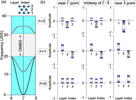
Figure 11. (a) The assumed trilayer structure in fcc(001) stacking and the magnon dispersion relation calculated based on a Heisenberg model along the  –
– –direction of the surface BZ. The assumption here is J⊥ = 1.5J and J∥ = J. (b) The amplitude of the magnon wave packets in different layers. The amplitude is normalised for a better representation. In each graph values of Aj (j = 1, 2 and 3 is the layer index, as shown in the upper panel of (a)) are normalised to the total value given by
  . The amplitudes are shown for three different points, near the
  -point (first row), in the midway of
  –
– (second row), and near the
  -point (third row). The magnon amplitude for the mode with n = 0 near the
  -point is identical in all three layers. This indicates the uniform precession of spins in all layers and their equivalent contribution to the FMR mode of the system. The magnon's amplitude in the middle layer decreases while moving from the zone centre towards the zone boundary. At the
  -point only the magnon amplitude in the bottom and top layer remains. This means that at this point the n = 0 magnon mode is localised entirely in these two layers. For the n = 1 magnon mode, the zero amplitude at the middle layer indicates one node in the central atomic layer. The magnon mode with n = 2 has the largest amplitude in the middle layer. The amplitude of this mode becomes the largest at the
  -point, meaning that this magnon mode is mainly localised in layer 2.
Download figure:
Standard image High-resolution imageThe discussion provided above is for atomically thin ferromagnetic layers. A model based on Heisenberg Hamiltonian in the exchange regime, together with a transfer-matrix treatment within the random-phase approximation has been developed in references [129–131] for periodic and quasi-periodic crystals. The model assumes thin films of different materials which are exchanged coupled and, in a similar way, predicts existence of several bands and also partial bandgaps in such structures.
2.4. The magnon lifetime
There are several mechanisms which determine the lifetime of spin excitations in ferromagnetic thin films and multilayers. Discussing all those mechanisms is out of the scope of the present topical review. For the sake of completeness we just briefly discuss the important aspects in this section. For an extended discussion we refer the reader to references [127, 132–143].
Generally in the limit of small momentum the magnon lifetime is given by the Gilbert term appeared in equation (1). For the uniform FMR mode with q = 0 the lifetime is governed by the spin–orbit coupling. In this case the phenomenological damping parameter (known as Gilbert damping) shall explain the magnon damping. However, in the case of ultrathin films and low-dimensional magnets, other processes such as two-magnon scattering may also provide additional channels for damping (see for example reference [135] and references therein. In addition to these mechanisms the extrinsic damping processes, such as scattering from defects, phonons, domain walls and impurities can also largely contribute to the magnon decay.
In the limit of exchange magnons the lifetime is determined by the decay of the collective excitations into the single particle Stoner excitations i.e., Landau damping [127, 144–147]. It depends strongly on the available Stoner states in the system. In low-dimensional systems, such as magnetic monolayers, the Stoner continuum may be very much different from that of the bulk ferromagnets and hence the lifetime of magnons in these systems can be very much different. For example consider a thin film of a ferromagnetic metal grown on a nonmagnetic metallic substrate. If the hybridisation of the electronic states of the magnetic film with the ones of the substrate is such that a large number of Stoner states are created near the Fermi level, the lifetime of magnons excited in the ferromagnetic film will be very short. This means that the presence of the nonmagnetic substrate provides an addition decay channel of collective magnon modes into single particle Stoner excitations. In other words, the energy and the angular momentum of the spin system is transferred by the conduction electrons of the underlying substrate. In case that the ferromagnetic film is not strongly hybridised with the underlying substrate it is expected that the magnons in the ferromagnetic film live for a much longer time.
The mechanism discussed above is mainly responsible for the damping of exchange magnons in metallic ferromagnets. One should note that there are also other sources for damping. For example one can imagine that a dephasing of a certain magnon mode with a given wavevector to all the other possible magnons with different wavevectors. Note that the damping of the magnons involve also the transfer of the angular momentum from the spin system to the lattice. Such a process requires a coupling mechanism which couples the spin system to the lattice. This coupling mechanism may be provided by the fundamental spin–orbit interaction.
3. Design of magnonic crystals
In section 2.3 we provided the fundamental concepts required to follow the topic of MCs. Now we review some of the selected recent experimental attempts for designing MCs operated in different frequency regimes with the emphasis on the physics of magnonic band structure, bandgaps and the magnon dynamics in these structures. We do not aim to discuss all the experimental results reported in the past two decades. For that we refer the reader to the existing reviews (see for example [148, 149])
3.1. Magnonic crystals for gigahertz magnons
Numerous attempts have been made in order to design periodic structures acting as MCs for gigahertz magnons. The physics of the magnons in these systems can be understood based on the concepts discussed in section 2.3.1. In such investigations typically one starts with a thin film of magnetic material and introduces modulations in one or two dimensions (for example square arrays of either disks or holes). The magnon dispersion relation is probed along the main symmetry directions of the first BZ of the artificial crystal, created in this way [49, 150–154]. The idea has even been extended to MCs made out of antiferromagnetic thin films [155].
As an example we show in figure 12 the magnon dispersion relation probed by Gubbiotti et al in an array of ferromagnetic stripes, representing one dimensional MCs [156]. Since in this case the stripes are coupled strongly via the dipolar interaction the dispersion relation exhibits the expected periodicity while going from the first to the second BZ. Furthermore, one observes the appearance of bandgaps between different magnon modes [156]. The experiments have been performed on two different sets of samples; one including stripes all having the same width and the other including stripes with different widths. It has been observed that the calculated dispersion relation, taking into account the dipolar coupling between the stripes, reproduces the experimental results. Several similar works have been performed by different groups [123, 157–164]. The experiments have been extended to bi-component stripes [165, 166].
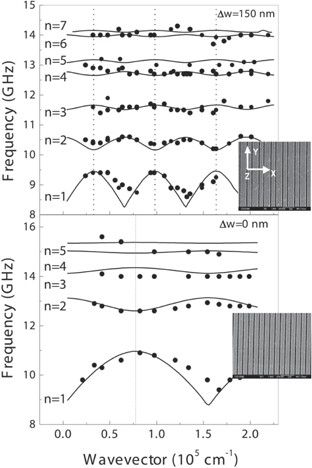
Figure 12. The magnonic band structure of a 1D MC composed of arrays of ferromagnetic stripes as probed by Gubbiotti et al [156]. A magnetic field of μ0H = 50 mT was applied along the stripes length. The SEM images of the studied structures are shown as insets. Δw refers to the width difference of neighbouring stripes. Upper panel shows the results of the sample consisting of stripes with different widths. The lower panel shows the results for stripes with identical widths. The zone boundaries are indicated by vertical dotted lines. Adopted from Gubbiotti et al [156]. Copyright (2007) by American Institute of Physics.
Download figure:
Standard image High-resolution imageIt is rather straightforward to find the origin of the formation of different modes in such a model system. When the stripes are magnetised parallel to their length the static magnetisation is either parallel or antiparallel to the strip. The dynamic dipolar stray fields caused by the precessing magnetisation of each stripe couples to the neighbouring one (the dynamical part of the magnetisation is perpendicular to the stripe). This coupling provides the relevant interaction which leads to the formation of magnons in the whole structure. The magnonic band structure is therefore governed by the shape of each stripe and also the coupling between different stripes. The intrinsic mode of each stripe is a confined mode with the lowest frequency. Now if one considers the boundary conditions, the amplitude of the dynamic part of the magnetisation is not constant across the width of the stripe. The boundary conditions depend on the mode number. The frequency of each mode is determined by the materials parameter and also the geometrical consideration of the sample. When the stripes are coupled via the dynamic dipolar stray fields, one observes the formation of minibands, which are separated by forbidden frequency gaps. The increase of the frequency of the first mode with the wavevector can be understood based on the following arguments. When the fundamental mode of the system is excited, at the centre of BZ the dynamical components of the magnetisation of neighbouring stripes precess with the same phase. However, at the zone boundary they precess with a phase difference of π. While in the former case the excitation of magnons demands a low energy, in the latter case a much higher energy is required to excite the magnons. Putting these two limits together one can intuitively understand the dispersive behaviour of the fundamental mode of the system. The energy of the mode is minimum at the zone centre and rapidly increases while changing the wavevector towards the zone boundary. This leads to a pronounced dispersive behaviour of the first mode. The dynamic dipolar coupling decreases with the mode number. Hence the higher order modes become less dispersive. With similar arguments one can explain the decrease in the band splitting while increasing the mode number.
Generally, details of the magnonic band structure of such a system depend on the coupling strength between the stripes. Such a coupling can be tuned either by changing the separation distance between stripes [167] or by changing the width of stripes [168]. The latter one shall also change the frequency and the shape of the intrinsic mode. Note that the frequency of the intrinsic mode of each individual stripe can be tuned by changing the materials parameter such as magnetisation, exchange stiffness constant, magnetic anisotropy as well as the geometrical parameters such as width, length and thickness.
As discussed in section 2.2 in the MSBVW geometry, where the magnetic field is applied in the direction perpendicular to the stipes, the demagnetising field is fully inhomogeneous across the stripe (see figure 6). This leads to the formation of localised edge modes as well as modes which are localised at the centre (centre modes). The edge modes can exhibit symmetric or antisymmetric profiles with respect to the centre of the stripe. The frequency of these modes depends on the coupling between the dynamical magnetisation at the edges. Such a coupling is of both dipolar and exchange nature. While the dipolar interaction favours an antisymmetric mode formation, the exchange interaction favours a symmetric mode. In case that the width of the stripe is large, so that the dynamical magnetisation at the edges are not coupled both the symmetric and antisymmetric modes degenerate. Details of the modes and their band dispersion depend on the material parameters and the geometrical structure. The width of the stripes and their separation distance are the variables, which can be used to tune the band structure.
Likewise in the MSFVW geometry the dynamical magnetisation of the stripes couples in the direction perpendicular to the stripes. Hence, assuming that the thickness of the stripes is much smaller than their width, one would expect to observe effects similar to those observed in the DE geometry [169]. Therefore, the magnonic band structure can be tuned in a similar way as in the case of the DE mode.
More recently the evolution of the magnon modes in the transition from a continuous thin film to a 1D MC has been investigated by means of FMR. The study provides some interesting details regarding the evolution of the modes when a thin film is smoothly transformed into an MC. Probing the transition states has been realised by a gradual decrease of the film thickness of the materials filling the regions between the stripes. It has been observed that in the transition region the uniform magnon mode of the film maintains as a groove mode in backward volume geometry and as a quasi-uniform mode in the DE geometry. The mode finally disappears when the system is developed to an MC. In the case of the MSBVW it has been found that the transition process is governed by the presence of strong magnetising and demagnetising fields which lead to the formation of 2n − 1 modes inside the stripes. In the case of the DE geometry the transition process is governed by the preservation of the natural wavelengths of the modes. As a consequence in the backward volume geometry the mode with the quantum number n evolves into the mode with the quantum number of 2(n − 1). In the DE geometry the modes with the odd quantum number evolve to modes with the quantisation number of n − 1 and those with the even value of n evolve to either modes with quantum number n or n − 2 [170].
As a general remark, since the bands of magnons propagating in the direction along the stripes would cover the regions of bandgap (along the direction perpendicular to the stripes), one would not expect full bandgaps in the case of 1D MCs [171–175].
The structures have successfully been extended in two dimensions [114]. The discussions provided above are also valid for the case of periodic structures in 2D, since the magnon characteristics obey, to a large extent, the same physics [176]. The most prominent examples of this kind are 2D dot [120, 177–186] and antidot lattices [115, 187–216] with various shape and Bravais lattices. Such structures have been investigates extensively and have already been reviewed (see references [210, 217, 218] for reviews). The idea have been extended to 3D [219–224] and coupled [225–231] MCs.
In addition to the idea mentioned above there has been other ideas to periodically modulate the magnetic properties (mainly the magnetisation) and thereby realise MCs. Examples of this kind are MCs realised by periodic current fellow on top of a magnonic waveguide or by means of periodic modulation of temperature via local heating. Even travelling [232–234] and dynamic MC [235–238] have also been realised based on a similar idea. We do not aim to discuss those in the present topical review (for details see for example reference [149] and references therein).
3.2. Magnonic crystals for terahertz magnons
As discussed in section 2.3.2, in an ultrathin film, the translational symmetry is broken in the direction perpendicular to the layers. This fact leads to the appearance of discrete magnon states with a quantised perpendicular momentum q⊥ = nπ/d. This means that modes with zero, one, and two half-wavelength envelopes of standing spin waves are confined inside the film. Consequently, spins between adjacent layers are no longer aligned parallel, and the modes with higher frequency are characterised by a larger deviation of the precession phase between adjacent layers.
The presence of the confined magnon modes with nonzero perpendicular momentum has been reported by means of scanning tunnelling spectroscopy (STM) [239, 240]. High-resolution electron energy-loss spectroscopy experiments on Co films have also shown the presence of the low-energy confined magnon modes mainly with (n = 1) near the centre of the Brillouin zone [241–244]. Since such magnons propagate in the x–y plane due to the presence of the translation invariance in the film plane, each mode shall have its own in-plane dispersion relation as a function of qx (qy). The magnonic band structure of such a system shall exhibit bandgaps as well as allowed magnon states (see figures 10 and 11). The full dispersion relation of the quantised magnon modes has recently been measured in a thin Co film composed of three atomic layers [245].
The magnonic band structure experimentally probed in a thin film of fcc Co grown on Cu(001) is shown in figure 13(a). The experimental data are shown together with the results of ab initio calculations, including spin-dependent many-body correlation effects. Details regarding the impact of the spin-dependent many-body correlations on the magnonic bands are not relevant for the present topical review and are discussed in reference [245]. One observes all the three expected modes as a result of quantum confinement in the structure. These modes exhibit several characteristics, as outlined below.
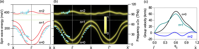
Figure 13. (a) The experimental and theoretical magnonic band structure in a thin film of fcc Co grown on Cu(001). The experimental data are shown together with the results of ab initio calculations, in which the spin-dependent many-body correlation effects are considered. The data are shown over the first surface BZ. (b) The Bloch spectral function of magnons for the same system. The spectral function is projected onto all three layers. The data are shown over the first and second surface BZ. (c) The group velocity of different magnon modes. Data are taken from Chen et al [245]. Copyright (2017) by the American Physical Society.
Download figure:
Standard image High-resolution imageThe first two modes with the lowest frequency (the modes with quantum numbers n = 0 and 1) are formed due to the presence of the top and bottom layers. A useful information from the ab initio calculations is the magnon Bloch spectral function in the frequency–momentum space. As discussed in section 2.3.2 the solution of the Heisenberg Hamiltonian can be represented as Bloch states, in analogues to the Bloch electronic states in solids. At a given momentum the spectral function shows peaks at the eigenfrequencies of different magnon modes sharing the same wavevector. In the case of Bloch electronic states an integration of the Bloch spectral function over the momentum provides the density of electronic states. Likewise, in the case of magnons their Bloch spectral function would provide the magnon density of states. This is of particular importance for separating the contribution of different layers to a specific magnon mode. We would like to emphasise that the Bloch spectral function calculated within this scheme does not account for the magnon damping. In this description it is assumed that all the magnon modes exhibit the same (weak) damping. The idea behind this representation is to show the localisation of different magnon modes in different parts of the structure. This idea originates from the Bloch spectral function of electronic states in solids. The band structure calculated within this formalism shows the position of the magnon bands in the frequency–momentum space and not their damping. The beauty of this approach is that one can project the magnon bands into different layers and thereby see how the magnonic band structure is formed. We will discuss this point later. Figure 13(b) represents the calculated magnons Bloch spectral function of 3 ML Co on Cu(001). The results are shown for the first and second BZ, indicating the perfect periodicity of the magnon band structure due to the presence of the translational symmetry in the film. The first two modes (modes with n = 0 and 1) exhibit a positive and rather larger group velocity. In contrary, the mode with n = 2 shows a rather flat dispersion and consequently a small group velocity. It acts as a nearly standing wave. Figure 13(c) presents the group velocity of the different magnon modes of the 3 ML Co/Cu(001) system. The group velocity vg is obtained according to the relation vg = ∂ω/∂q∥. In addition to the fact that the group velocity of the n = 2 magnon mode is rather low, it also exhibits a sign change while increasing the wavevector from q∥ = 0 towards the zone boundary ( -point).
The n = 2 magnon mode is separated from the other modes with a rather large OMBG. In the present case this bandgap is on the order of 90 meV (∼22 THz). This large OMBG is a consequence of the strong coupling of the middle layer to the top and bottom layers [see also figure 10(c) and the related discussions in section 2.3.2].
The dispersion relation and consequently the group velocity of different magnon modes can be tuned via changing the interatomic exchange parameters or the geometrical structure of the system. In the case of n = 2 magnon mode, since the frequency is mainly governed by the interlayer exchange interaction, representing the coupling of the middle layer to the top and bottom layers, the mode is very sensitive to changes in these quantities. In order to demonstrate such an effect, in the first step, one may prepare two nearly identical samples, one with cubic fcc structure and another one in tetragonally distorted structure (face-centered tetragonal, fct). In the next step one can prepare the same sample in two different geometrical structures e.g., one with (001) stacking and the other one with (111) stacking. Thanks to advances in ultrathin film fabrication technology. Preparing such samples is possible by the right choice of the substrate. The idea has been realised by growing a Co film on different substrates [245].
Note that in the above discussion for simplicity we reduced the role of the substrate to change only the geometrical structure of the ferromagnetic film grown on top. This assumption is only valid when the electronic states of the film and substrate are decoupled. Such an assumption is not valid in real systems, in particular when the ferromagnetic film is grown on a metallic substrate. The strong hybridisation of the electronic states of the film with those of the substrate alters the magnetic properties of the film. In particular the magnetic exchange interaction in the atomic layer next to the substrate will be modified in the presence of such strong electronic hybridisations. The electronic hybridisations may even change the character of the exchange interaction (for example an antiferromagnetic exchange interaction may be favoured, instead of a ferromagnetic one [246]). Hence, the pattern of the exchange interaction across a ferromagnetic film grown on a nonmagnetic substrate can be rather complicated (for a review see for example [247]). Another important remark is that, we assumed that a decrease in the distance between layers leads to an increase in the interlayer exchange coupling. One should note that the change in the interlayer distance can lead to the renormalisation of the electronic structures of the system and consequently change the whole pattern of the exchange parameters (both the inter- and intralyer coupling) [128]. One therefore has to bare in mind that there is no simple rule of thumb to easily predict the behaviour of the inter- and intralayer exchange parameters while changing the interatomic distances of magnetic atoms in metallic ferromagnets. In other words the inter- and intralayer exchange parameters are interconnected in a rather complex manner. Consequently, for an accurate prediction of the evolution of the inter- and intralayer exchange parameters with changing the interatomic distances ab initio calculations are required. Such calculations provide valuable insights into the physics of the system [128, 245, 248].
In figure 14 the magnon band structure probed in a thin Co film composed of three atomic layers grown on different substrates e.g., Cu(001), Ir(001) and Pt(111) is shown. The results are accompanied with the results of ab initio calculations. Although all three systems exhibit a semi-parabolic dispersion relation for the n = 0 and n = 1 magnon bands, the shape of the dispersion relation of the n = 2 mode is different for different systems. This mode shows a downward parabolic shape for Co/Ir(001) and an upward parabolic shape, in the case of Co/Pt(111). This is in contrast to the nearly flat dispersion relation observed for the Co/Cu(001) system. The results confirm that the dispersion relation of the confined magnon modes is extremely sensitive to small changes in the lattice structure as a result of the film epitaxy. Hence, the film epitaxy can be used as a tool to tune the magnon band structure in epitaxial systems.
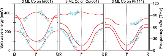
Figure 14. (a) The experimental and theoretical magnonic band structure in a thin film of fcc Co grown on different surfaces Ir(001) (left), Cu(001) (middle), and Pt(111) (right). The experimental data are shown together with the results of ab initio calculations, in which the spin-dependent many-body correlation effects are considered. The data are shown over the first surface BZ. Data are taken from Chen et al [245]. Copyright (2017) by the American Physical Society.
Download figure:
Standard image High-resolution imageWhile in the case of Co/Cu(001) the Co films grow in a nearly perfect fcc like structure, in the case of Co/Ir(001) the films grow in fct structure with a rather larger tensile stress. This means that in the former case one deals with a rather isotropic exchange interaction through the film (J∥ ≃ J⊥). In the latter case the exchange interaction is anisotropic (J∥ < J⊥). The anisotropy in the exchange parameters comes from the fact that the interatomic distances in the direction perpendicular to the layers is smaller than the interatomic distances in the plane. The interlayer exchange parameter is therefore larger than the interalayer one. Under such conditions one expects characteristic differences in the dispersion relation of the n = 2 magnon mode of the system, as discussed using a simple Heisenberg model in section 2.3.2. This fact has been confirmed by ab initio calculation. The ab initio results further indicate that the electronic states of Co film hybridise with the ones of the underlying metallic substrate, leading to layer-dependent and anisotropic exchange parameters. Such an effect has been observed in several cases [128, 140, 242, 245, 249–252]. The magnon band structure is modified not only due to the changes in the geometrical arrangement of atoms but also due to the hybridisation effects of the electronic states of the film with those of the substrate. This fact may be used as an additional tool to tune the magnonic band structure in a desired manner.
Comparing the results of the Co films in (001) stacking to those of the Co/Pt(111) system, indicates that one can even change the shape of the dispersion relation by changing the geometrical arrangement of atoms. The dispersive behaviour of different magnon modes reflects the propagation characteristics of these modes. Again of particular interest is the n = 2 magnon mode. Since this mode is a direct consequence of the strong coupling of the middle layer to the top and bottom layers, this mode is mainly localised in the inner layer. In this sense it might be regarded as a volume mode originating from the interior part of the film. The group velocity of this mode is positive for the Co/Pt(111) system, small for Co/Cu(001) and negative for the Co/Ir(001) system. Hence it acts a forward volume mode for the case of Co/Pt(111), as a quasi-standing wave in the case of Co/Cu(001) and as a backward volume mode in the case of Co/Ir(001).
Next let us discuss the possibility of tuning OMBG opened between the n = 1 and n = 2 magnon modes. Since the magnon band structure is governed by the interatomic exchange parameters a way to tune the bandgap is to change these parameters. The position and the size of the OMBG could indeed be tuned by varying the inter- and intralayer exchange parameters via changing the lattice distortion and the interfacial electronic hybridisations. This has been demonstrated by growing a Co film of the same thickness on the Ir(001) and Rh(001) surfaces. The lattice parameter of Ir (Rh) is about 3.84 (3.80) Å. Hence when Co film is grown on these substrates the tetragonal distortion of the lattice is rather large. In addition the interfacial electronic hybridisations of the Co/Ir and Co/Rh interfaces are stronger than those of the Co/Cu interface. For example in the case of Co/Rh the size of the OMBG has been found to be about 100 meV (24 THz) within the energy window of 262–362 meV. The OMBG may also be tuned by adding another atomic layer. An illustration of this idea is provided in figure 15. The number of the confined magnon modes increases as the number of layers increases. The modes become more dense in frequency and hence the OMBG decreases.
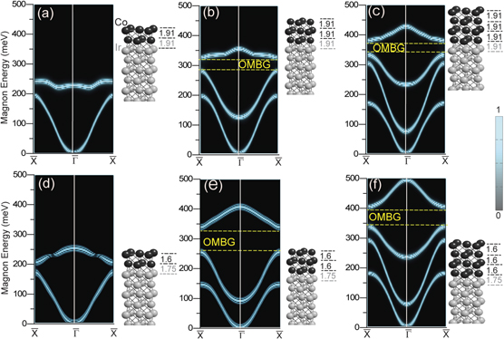
Figure 15. Illustration of the possibility of tuning the magnon band structure in atomically flat multilayers. The calculated magnon band structure of two [(a) and (d)], three [(b) and (e)], and four [(c) and (f)] atomic layers of ferromagnetic Co on Ir(001). The calculations have been performed based on ab initio density functional theory. The geometrical structure and the values used as the interlayer distances, given in angstrom, are drawn for each case. The results presented in the upper row are based on the assumption that the Co film grows in a perfect fcc like structure (with the same lattice parameter as the one of Ir in all three dimensions). The results shall show only the impact of the film thickness on the OMBG and exclude the role of the tetragonal distortion. In (d)-(f) the effect of the tetragonal distortion has been taken into account by using the experimental interatomic distances as the input of ab initio calculations. Adopted from Qin et al [126]. Copyright (2019) by the American Physical Society.
Download figure:
Standard image High-resolution imageFigure 15 provides a summary of the gap opening in the magnonic band structure of the layered structures and the possibility of its tuning. The magnonic band structure calculated for the cubic [figures 15(a)–(c)] and tetragonally distorted [figures 15(d)–(f)] films is shown. The calculations are performed for 2–4 ML Co on Ir(001). The OMBG is opened for the 3 and 4 ML samples. The tetragonal distortion leads to an increase in the value of OMBG [compare figures 15(b) and (e)]. In the case of a 4 ML film the OMBG appears between the n = 2 and n = 3 magnon modes and is smaller than the sample composed of 3 ML [compare figure 15(b) to (c) and (e) to (f)]. Furthermore, one notices that adding an additional layer to the system leads to a shift of the OMBG towards higher frequencies.
The next question to answer is whether it is possible to open a bandgap between the n = 0 and n = 1 magnon bands. Such a bandgap may be called an acoustic-optical magnon bandgap (AOMBG). Since the first two magnon modes possess a large group velocity, utilising these magnons would be of the interest for ultrafast magnonics. As discussed in section 2.3.2 these two modes are the consequence of the broken inversion symmetry at the top and bottom surfaces. Since atoms sitting in these two layers possess less neighbours, compared to the atoms sitting in the inner part of the film, these modes exhibit lower frequencies. In order to be able to open a bandgap between the n = 0 and n = 1 magnon bands, it is essential to unravel the origin of these magnon bands and find the places in the structures where these magnon modes are localised. In the language of classical spin dynamics the localisation of a certain modes means that the dynamical part of the spins located in one particular part of the structure has a larger amplitude when the corresponding collective mode of the system is excited. Such information can be extracted from the analysis of the Bloch spectral function of magnons. If the top and bottom layers are magnetically identical, the spins sitting in these two layers will equally contribute to these two modes. One would expect these modes to degenerate at the zone boundary. In other words it is not possible to associate one mode to one layer. In the case of thin films grown on a substrate the top and bottom layers are no longer equivalent. This leads to differences in the pattern of the Bloch spectral function, of these modes and the spatial localisation of the modes. The differences become more visible when the hybridisations of the electronic states of the film with those of the substrate become stronger. Hence, one would expect a larger degeneracy-breaking for films grown on substrates with stronger electronic hybridisations. Examples of such substrates are transition metals with empty states in the d band e.g., Ir, Rh, Pt, etc.
Such analyses of the magnon Bloch spectral functions have been performed in references [126, 248, 253]. In figure 16 the example of 3 ML Co/Ir(001) is provided. The calculations have been performed based on first principles (for details see reference [245]). The spectral function projected onto all three layers is presented in figure 16(a). The magnon density of states (DOS) calculated by integrating the Bloch spectral function over q∥ is shown in the right side. The magnon DOS exhibit an OMBG in the range of 262–362 meV (63–88 THz). The magnon DOS exhibits peaks near the bottom and top of each magnon band. The projected Bloch spectral function onto the interface, middle and surface layer is shown in figures 16(b)–(d). The partial magnon DOS is shown in the right side of the spectral function in each case. Both the projected Bloch spectral function and the layered resolved magnon DOS indicate that the magnon mode with n = 0 is mainly localised in the interface layer. Likewise the n = 1 and n = 2 modes are mainly localised in the surface and middle layers, respectively.
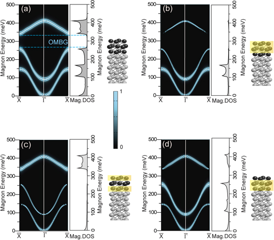
Figure 16. (a) The magnon Bloch spectral function and the magnon DOS projected onto all three layers of fcc Co(001) film on Ir(001), as calculated based on first principles. The magnon Bloch spectral function as well as the magnon DOS projected onto the interface atomic layer (b), the middle layer (c), and the surface layer (d). The n = 0 magnon mode has the largest spectral weight and DOS when it is projected onto the interface layer. Data are taken from Qin et al [126]. Copyright (2019) by the American Physical Society.
Download figure:
Standard image High-resolution imageThe behaviour discussed above has been observed for many combinations of ferromagnetic thin films grown on nonmagnetic substrates. The general observation is that the n = 0 magnon mode is mainly localised in the interface layer (the one next to the substrate), where the exchange parameters are smaller. Consequently the n = 1 magnon mode is mainly localised in the surface layer. As another consequence of the smaller exchange parameters in the interface layer one observes that the frequency of this mode reduces. Hence, it is, in principle, possible to design a system in which the n = 0 magnon mode lies fully below the n = 1 magnon mode.
The key idea to open an AOMBG is to take advantage of competing exchange interaction between nearest and next nearest neighbour spins in the interface layer. Based on a simple Heisenberg model one can show that the material of choice for the interface atomic layer should fulfil the following conditions. (i) Since the dispersion of the n = 0 magnon mode is mainly governed by the intralayer exchange parameters in the interface layer, this interaction shall be weak to reduce the frequency of this mode. In order to illustrate the role of competing magnetic interaction, let us consider again the trilayer structure discussed in figure 10(d). Opening an AOMBG would mean that the frequency of the n = 0 mode at the high-symmetry  - and
- and  -points shall be smaller than the one of the n = 1 magnon mode at the
  -point. Considering only the nearest neighbour exchange interaction the bandgaps are given by
 ![${{\Delta}}_{\bar{{\Gamma}}-\bar{\mathrm{X}}}^{\mathrm{A}\mathrm{O}\mathrm{M}\mathrm{B}\mathrm{G}}=\left(1/2\pi \right)\left[{\omega }_{n=1}\left(\overline{{\Gamma}}\right)-{\omega }_{n=0}\left(\overline{\mathrm{X}}\right)\right]=-8{J}_{\parallel }S/h$](https://content.cld.iop.org/journals/0953-8984/32/36/363001/revision2/cmab88f2ieqn54.gif) and
and ![${{\Delta}}_{\bar{{\Gamma}}-\bar{\mathrm{M}}}^{\mathrm{A}\mathrm{O}\mathrm{M}\mathrm{B}\mathrm{G}}=\left(1/2\pi \right)\left[{\omega }_{n=1}\left(\overline{{\Gamma}}\right)-{\omega }_{n=0}\left(\overline{\mathrm{M}}\right)\right]=-16{J}_{\parallel }S/h$](https://content.cld.iop.org/journals/0953-8984/32/36/363001/revision2/cmab88f2ieqn55.gif) for the
for the  and
and  directions, respectively. This implies that the value of J∥ should be negative, in order to have a bandgap opened. However, one has to note that if J∥ is negative in all layers it will change the shape of the n = 1 mode and consequently there will be no bandgap. Hence, only when the intralayer exchange parameters are different in different layers one would be able to open an AOMBG. Furthermore, not only the nearest neighbours but also the next nearest neighbour interactions become important. A competition between the exchange parameter leads to an AOMBG. (ii) The next nearest neighbour exchange parameter shall be smaller than the nearest neighbour one. This is usually the case for metallic ferromagnets. If the next nearest neighbour exchange interaction is of antiferromagnetic character it will be an advantage, because this leads to a reduction of the magnon energies near the zone boundary [246]. (iii) Since the frequency of the n = 1 magnon band at the zone centre is governed by the interlayer exchange interaction, this exchange constant should be large enough to keep the n = 1 magnon band at higher frequencies, above the n = 0 magnon mode. The first two conditions can be satisfied by taking advantage of the interfacial electronic hybridisations of the ferromagnet film with the metallic substrate, the last condition may be satisfied by tuning the interlayer spacing and taking advantage of epitaxial growth and tetragonal distortion of the ferromagnetic film.
As pointed out above, it is well-known both theoretically and experimentally that when ultrathin Fe films are grown on 4d or 5d metallic substrates, at the interface the electronic states of the film hybridise rather strongly with those of the substrate [142, 246–248, 253–255]. This fact leads to a weakening of the exchange interaction in the interface atomic layer. If the film is grown on a crystal with a larger lattice constant (compared to the lattice constant of the film), the next nearest neighbour exchange constant has a tendency to be of antiferromagnetic character (negative exchange constant) and in some cases its strength (absolute value) is comparable to the nearest neighbour exchange constant [246, 247]. It means that in order to realise such an idea the material of choice for the first (and maybe the second) atomic layer should be Fe and the film should be grown on a crystal with a larger lattice parameter.
The realisation of an AOMBG has recently been reported in reference [126]. Several synthetic layered structures have been examined. The magnon band structure of a structure composed of one atomic layer of Fe and two atomic layers of Co has been found to exhibit an AOMBG on the order of 25 meV (6 THz). Figure 17 summarises the results of the magnon band structure measured in this system. The observed AOMBG is located between the bottom of the n = 1 magnon band at the  -point and the top of the n = 0 magnon mode in the midway of
  –
– direction.
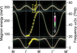
Figure 17. The magnonic band structure of a thin ferromagnetic film composed of two atomic layers of Co, one atomic layer of Fe grown on Ir(001). The experimental results are shown by open symbols and the results of modelling based on a Heisenberg model are presented as the spectral function projected onto all layers. The band structure is shown over the first and second BZ, indicating the presence of the translation symmetry in the film plane. The Data are taken from Qin et al [126]. Copyright (2019) by the American Physical Society.
Download figure:
Standard image High-resolution imageAs a side remark, based on the same idea one may propose a similar design strategy for designing a three dimensional magnonic crystals suitable for operations at lower frequencies (sub-terahertz). Essentially, in such a case the atomic layers should be replaced by magnetic films with a thickness of a few nanometers. In addition one should replace the direct Heisenberg exchange with the indirect Ruderman–Kittel–Kasuya–Yosida (RKKY) interaction [256–258]. This might be realised by introducing a nonmagnetic spacer layer between the ferromagnetic films. Such multilayer structures may be patterned in any desired periodic form and the empty spaces may be filled again with the same nonmagnetic material used for the spacer layer. The key point is that the magnetic elements should be exchange coupled.
3.3. Other types of magnonic crystals
Recently, other types of MCs have also been proposed. The core fundamental idea behind the design strategy is very similar to that of the MCs discussed in sections 2.3, 2.3.1 and 3.1. However, there are also fundamentally interesting new physics that leads to the new properties of these MCs.
3.3.1. Magnonic crystals with periodically modulated Dzyaloshinskii–Moriya interaction
Dzyaloshinskii–Moriya interaction (DMI) is an antisymmetric magnetic interaction originating from spin–orbit coupling in the absence of inversion symmetry. This interaction has the form of  , where Dij is the so-called microscopic DMI vector. It has been shown that DMI modifies the properties of magnons in chiral magnets [247]. The most prominent effects of DMI on the magnon dispersion relation is that it leads to an asymmetry in the dispersion relation [259] and the magnon lifetime [136]. These effects result in a nonreciprocity in the propagation characteristics of counter propagating magnons. Recently, it has been proposed that a periodic modulation of this interaction leads to very interesting effects on the magnonic band structure of gigahertz magnons [50]. Analytical calculations combined with micromagnetic simulations have revealed the interesting features of the magnon band structure in these systems e.g., indirect magnonic bandgaps. Furthermore, several interesting effects such as dispersionless bands have been observed in the simulations. As the presence of the DMI leads to the nonreciprocity of magnons, this leads to unusual temporal behaviour of standing spin waves, exhibiting nonzero phase velocities (for a review on the topic see chapter 5 of reference [19]).
3.3.2. Magnonic crystals based on topological defects
As pointed out in section 2.3.1 periodic spatial modulation of any magnetic parameter may be used to design MCs. Such modulation may be done on the domain pattern of a thin film [260, 261] or periodic magnetic vortices [262, 263]. Likewise this may be realised by introducing ordered topological defects in the system. Based on numerical simulations Ma et al have demonstrated a novel MC based on a linear array of skyrmions [54, 264–266]. Skyrmions are nanoscale topological spin textures emerging in some chiral magnets. A magnetic stripe, acting as a waveguide, with 1D arrangement of skyrmions has been considered. It has been shown that the skyrmion-induced spatial variation of the magnetisation along the waveguide results in a drastic modification of the magnon dispersion relation, which leads to the appearance of allowed and forbidden bands in its band structure.
The numerically obtained magnonic band structure by Ma et al [54] in the 1D periodic skyrmion lattice formed in a waveguide is presented in figure 18(a) in the extended zone scheme. The band structure exhibits a periodic character of the three BZs. Back folding of the bands into the first BZ would results in bandgaps with the magnitude of 6, 4, and 2.5 GHz. It has been also illustrated that magnons in such a system exhibit nonreciprocity due to their chiral nature. The nonreciprocal behaviour of these magnons is demonstrated in figures 18(b) and (c), where the magnon amplitudes at the two edges of the waveguide are presented as the colour scale. On the edges of the waveguide the counter-propagating magnons are localised. This means that the magnons travelling to one side of the waveguide are localised at one edge and those travelling to the opposite direction are localised in the other edge of the waveguide. The chiral character of these magnons originates from DMI.
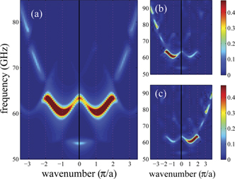
Figure 18. The magnon dispersion relation in a skyrmion based magnonic waveguide composed of a linear array of skyrmions, as calculated by Ma et al [54]. The dispersion relation at the centre of the waveguide is presented in (a). The dispersion relation at the two edges are shown in (b) and (c). The dashed vertical lines indicate the BZ boundary. The magnon intensity is shown by the colour scale, indicating that at the two edges of the waveguide counter-propagating magnons travel. Reproduced with permission from Ma et al [54]. Copyright (2015) by the American Chemical Society.
Download figure:
Standard image High-resolution image
Such a skyrmion-based MC is dynamically reconfigured by changing the diameter of the skyrmions e.g., by applying a current, and bias magnetic or electric field [54]. The same may be realised by changing the periodicity of the lattice using external stimuli.
In a 2D lattice of ferromagnetic as well as aniferromagnetic skyrmions it has been shown that one would expect to observe a very interesting magnonic band structure containing allowed magnon bands, bandgaps as well as chiral edge states, which are topologically protected [267, 268], similar to those in topological magnon insulators [269].
The idea may be extended to 3D skyrmion crystals. In bulk chiral magnets the skyrmion lattices are usually stabilised by temperature and application of a magnetic field. It has been shown that the dynamics of such systems do not obey the dynamics of a simple ferromagnetic sample given by equations (2)–(4). The FMR response of such systems has been investigated in detail [270]. It has been observed that in the skyrmion phase there exist three magnon modes describing clock wise motion, counter clock wise motion and breathing of the skyrmions. A generalised description of the resonance frequency has been reported for materials hosting skyrmion crystals through the whole phase diagram [270]. Furthermore, it has been illustrated that such MCs would allow for nonreciprocal microwave components and grating couplers controlled by external stimuli (for review see for example reference [271]). This is a promising research direction that requires further experimental efforts for realisation of the effects predicted by the theory and simulation.
3.3.3. Magnonic crystals by incorporating Abrikosov vortices
It has recently been demonstrated that magnons excited in a thin ferromagnetic film can be coupled to a flux lattice of a thin superconducting film, if these two are brought in a close proximity. Experiments on Py/Nb bilayers have shown that the magnonic band structure of such a system contains allowed states as well as forbidden gaps, which can be tuned by a magnetic field. In addition the Doppler shifts in the frequency spectra of magnons scattered on a flux lattice has been observed when the lattice was moved by sending an electrical current through the superconducting layer [53].
4. Applications, major obstacles and possible solutions
4.1. Applications
One of the driving forces behind exploring MCs has been their possible application in the field of magnonics as platforms for control and manipulation of magnons or as devices with new functionalities [272–276]. Indeed proof of principles indicating the feasibility of using MCs for transfer, processing as well as buffering of analog and digital information has been reported in several experiments. MCs have been successfully implemented as microwave filters and resonators, microwave signal generators, frequency invertor, elements for data buffering, magnon transistors and other logic devices. Reviewing of all those results is out of the scope of the present topical review. The reader is referred to the existing reviews on this subject, for example see references [15, 149]. This is an intriguing research direction and there is still a lot of research to be conducted in this area.
4.2. Reconfigurability of magnonic crystals
One of the concepts which has been discussed in the context of MCs is their reconfigurability. In 1D MCs made of regular arrays of magnetic stripes the initial configuration of the static magnetisation pattern of the MC can be either parallel or antiparallel (considering only the shape anisotropy). If one considers other anisotropy terms, the pattern can be more complex. This initial state has direct consequences on the magnonic band structure of the system. MC can therefore be reconfigured by changing the magnetisation pattern. The same idea can be extended to more complex patterns and also to 2D MCs. One can realise different magnetisation patterns by different means such as magnetic/electric fields, electrical currents etc. With this one can eventually define the functionality of the device [277–282].
4.3. Challenges and solutions
4.3.1. Magnon lifetime
One of the main challenges hindering the application of MCs in practical devices is the lifetime of magnons [102, 283–288]. While in the case of ferromagnetic insulators the magnon lifetime is reasonably long, in most of the metallic ferromagnets magnons suffer from damping. In order to overcome this problem two alternatives have been suggested. First, efforts have been devoted to grow high quality thin films of magnetic insulators (mainly YIG films) with low damping [289] and use them further for nano-patterning and device fabrications [290]. Although fabrication of nano-elements based on ferromagnetic insulators is another challenge, the long magnon lifetime and several decade of research on these materials have made them still as the prime candidate for magnonic devices. Second, efforts have been devoted to suppress the magnon damping in metallic ferromagnets either by tuning the damping parameter through the modification of the material's property or by extrinsic effect such as magnon amplifications and exploiting the antidamping phenomena [11, 291–294]. Third, it has been suggested that by increasing the magnon group velocity one may enhance the mean-free-path of magnons and thereby overcome effect of damping [295].
The magnon damping is still a challenge in the case of terahertz magnons. The damping of terahertz magnons in itinerant ferromagnets is a result of their decay into Stoner excitations. Generally the probability of decay of a magnon to a Stoner pair can depend nonmonotonously on the frequency and wavevector. This behaviour in ultrathin ferromagnets and low dimensional magnetic structures can be very much different from that in the bulk ferromagnets. A way to gain a detailed knowledge on the Landau damping of terahertz magnons in itinerant ferromagnets is to calculate the Landau map. The concept has been introduced and discussed in references [144, 145, 147, 296]. It has been shown that by calculating the Landau map one can assess the contribution of different electronic states of the system to the Landau damping of magnons. Generally, the map provides direct information about the probability and the number of Stoner transitions, which contribute to the damping of a magnon with a given wavevector and frequency, over BZ. Places in BZ where the Stoner transitions happen with a large intensity are the hot spots. In the systems for which the number and the intensity of the Landau hot spots are larger the Landau damping is stronger. Hence, an efficient way to suppress the damping would be to modify the electronic band structure of the sample such that the intensity and the number of such hot spots are drastically reduced in the system. This idea has been realised for example in the case of an ultrathin Fe film alloyed with Pd [147].
On the other hand one should notice that the terahertz magnons possess a rather high group and phase velocity [see for example figure 13(c)]. Hence, although the damping parameter of terahertz excitations may seem to be high compared to the Gilbert damping parameter of the FMR mode, one may try to take advantage of the high group and phase velocity of terahertz magnons. The mean-free-path of a magnon wave packet is given by λ = vg ⋅ τ, where τ denotes the lifetime. In addition, the wavelength of terahertz magnons is rather short (it is on the order of interatomic distances, being a few Å). This fact enables scaling of the devices down to the atomic scales.
4.3.2. Excitations and detection
Magnons with a long wavelength (mainly dipolar and dipolar-exchange magnons) can be very efficiently excited and detected using microwave and optical techniques, methods based on electrical transports or combinations of these. Techniques like FMR, both in conventional and broad-band scheme provide excellent opportunities to excite and detect magnons near the zone centre. BLS and time-resolved optical methods provide frequency, wavevector, time, space and phase resolved measurement of long wavelength magnons. The recently developed techniques such as spin-torque- or spin-Hall-nano-oscillators have contributed very largely to the realisation of all electric magnon excitation and detection in magnonic devices (see for example [297, 298]). This has pushed the development in the field one big step further with the perspective of integrating the magnonic circuits with the current state-of-the-art spintronic technologies [299, 300]. However, in the case of terahertz magnons with short wavelengths one still needs to develop techniques for excitation and detection of these excitations. Spin-polarised high-resolution electron energy-loss spectroscopy (traditionally called spin-polarised electron energy-loss spectroscopy) has been used for fundamental investigation of such magnons in low-dimensional magnetic structures [248, 301–309]. The technique provides the magnonic band structure in a momentum-resolved manner with a high momentum resolution an extremely high sensitivity. Several interesting effects have already been observed using this technique [68, 126–128, 136, 142, 143, 147, 245–247, 251, 253, 254, 259, 296, 308–311]. Alternatives excitation schemes, which may enable the practical use of terahertz magnons in logic devices are as follows. Terahertz magnons can be excited by e.g., terahertz radiations (see for example see [312–314]), using nonlinear effects, spin torque nano-oscillators [11, 315] or very recently demonstrated vortex core excitation method [316]. The latter method allows coherent excitation of short wavelength excitations down to 80 nm wavelength (but still in gigahertz regime). The mechanism of magnon excitations in this case has been explained in terms of the mechanism initially introduced by Schlömann [84, 85, 317, 318]. In addition is has been demonstrated that terahertz magnons can be very efficiently excited in tunnelling junctions [319] and by electron tunnelling via an STM tip (see for example [240] and references therein). In these ways one may be able to excite terahertz magnons for application in logic elements. However, the first important step towards any future device application is the proof of concepts. Realisation of the concepts for practical applications is another challenge, which demands further efforts.
5. Summary and outlook
The characteristic properties of magnons in low-dimensional magnetic structures has opened possibilities to design structures, which may act as platforms for magnonics. Numerous experimental and theoretical works have demonstrated such possibilities, using different approaches. MCs, exhibiting allowed and forbidden bands at different frequency regimes, have been realised. For gigahertz frequency regime periodic modulation of the magnetic properties on micro- and nanometer length scales results in a rich magnonic band structure, which can be tuned in a desired way via changing the material parameters, the geometrical structures or external stimuli such as electric current, magnetic and electric fields.
New types of MCs based on periodic topological defects and periodic modulation of DMI have been suggested. In addition to the properties expected for magnons in MCs, in these structures novel phenomena are expected to be observed. Examples of such phenomena are emergence of topological magnons, nonreciprocal magnon states and unconventional magnon bandgaps. These novel phenomena are related to the chiral nature of magnons in such structures, as a consequence of active DMI [320].
In the less-explored terahertz frequency regime the quantum confinement of magnons in atomically flat thin films and multilyares leads to very interesting characteristics of terahertz magnons. These properties may be utilised for designing terahertz magnonic platforms. Since these excitations are governed by the magnetic exchange interaction, quantum engineering of this fundamental magnetic interaction is required in order to manipulate the magnonic band structure of terahertz magnons in a desired way. This has been realised by engineering of the geometrical lattice structure and/or the electronic properties of magnetic thin films. This allows one to tune the intrinsic properties of these magnons such as group and phase velocity. Furthermore, the magnonic band structure with allowed magnon states as well as forbidden gaps could be realised in synthetic layered ferromagnets.
Several magnon based devices have been proposed and experimentally realised. However, a large part of the activates are devoted to the magnons with gigahertz frequencies. Utilising exchange-dominated magnons would open possibilities for operations in terahertz frequencies and also would allow for further miniaturisation of magnon-based devises. For that the physics of terahertz magnons should be understood in great details and further novel experimental schemes for excitation and detection of these magnons should be developed. In the next step the existing challenges should be addressed, and finally possible proof of principle needs to be provided.
Acknowledgments
The author would like to gratefully thank J Kirschner for numerous discussions on the topic of spin excitations using spin polarised electrons. Thanks to all the former members of the SPEELS team at the Max Planck Institute of Microstructure Physics as well as to the former and current members of the Heisenberg Spin-dynamics Group at the Physikalisches Institut, Karlsruhe Institute of Technology, for their contribution to some of the experimental results discussed here. Fruitful collaborations and discussions with A Ernst are gratefully acknowledged. Most of the ab initio calculations discussed here were performed within these collaborations. We would like to also thank the Physikalisches Institut for hosting the group and providing the necessary infrastructure. This work has been supported by the Deutsche Forschungsgemeinschaft (DFG) through the Heisenberg Programme ZA 902/3-1 and ZA 902/6-1 and the DFG Grant No. ZA 902/4-1.