
Abstract
The elastic and anelastic properties of a single crystal of Co-doped pnictide Ba(Fe0.957Co0.043)2As2 have been determined by resonant ultrasound spectroscopy in the frequency range 10–500 kHz, both as a function of temperature through the normal-superconducting transition (Tc ≈ 12.5 K) and as a function of applied magnetic field up to 12.5 T. Correlation with thermal expansion, electrical resistivity, heat capacity, DC and AC magnetic data from crystals taken from the same synthetic batch has revealed the permeating influence of strain on coupling between order parameters for the ferroelastic (QE) and superconducting (QSC) transitions and on the freezing/relaxation behaviour of vortices. Elastic softening through Tc in zero field can be understood in terms of classical coupling of the order parameter with the shear strain e6, λe6 , which means that there must be a common strain mechanism for coupling of the form λ
 QE. At fields of ~5 T and above, this softening is masked by Debye-like stiffening and acoustic loss processes due to vortex freezing. The first loss peak may be associated with the establishment of superconductivity on ferroelastic twin walls ahead of the matrix and the second is due to the vortex liquid–vortex glass transition. Strain contrast between vortex cores and the superconducting matrix will contribute significantly to interactions of vortices both with each other and with the underlying crystal structure. These interactions imply that iron-pnictides represent a class of multiferroic superconductors in which strain-mediated coupling occurs between the multiferroic properties (ferroelasticity, antiferromagnetism) and superconductivity.
Export citation and abstract BibTeX RIS

Original content from this work may be used under the terms of the Creative Commons Attribution 3.0 licence. Any further distribution of this work must maintain attribution to the author(s) and the title of the work, journal citation and DOI.
1. Introduction
One of the significant achievements of the 20th century was the discovery of high Tc cuprate superconductors which allow electrical conductivity with zero resistance at liquid nitrogen temperatures. In a quite different context, but with equivalent impact, there has been intense interest in multiferroic materials, defined as those displaying at least two out of ferroelastic, (anti)ferromagnetic and ferroelectric properties. The latter will be used for device applications, such as memories, with external control by combinations of magnetic, electric and stress fields. In both cases, the underlying physics is that the functional properties of interest are related to the proximity of multiple instabilities. The scientific challenge is to determine relationships between structure and properties for the individual instabilities and then to explore composition space to find where they can be arranged to converge in multicomponent solid solutions.
Unconventional superconductors can define a distinct class of their own as 'multiferroic superconductors' when the ferroic transitions are linked with unconventional superconductivity, as illustrated schematically in figure 1, following Carpenter [1]. One example of a ferroelastic superconductor without spin order is FeSe [2], and an example of a homogeneous superconductor which is also both ferroelastic and antiferromagnetic is underdoped Ba(Fe1−xCox)2As2 (x < ~0.06; e.g. [3–6]). Static magnetic order disappears in overdoped samples (x > ~0.06) but they still display evidence of favourable coupling between spin fluctuations and superconductivity [7, 8].
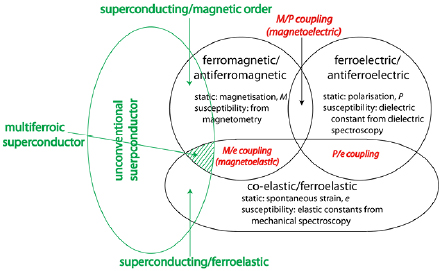
Figure 1. Relationships between ferroic properties in terms of coupling effects (after [1]) and their overlap with unconventional superconductivity. The hatched region defines the field of multiferroic superconductivity to which iron based superconductors such as Ba(Fe0.957Co0.043)2As2 belong.
Download figure:
Standard image High-resolution imageAn additional and inevitable consequence of overlapping instabilities is that they can give rise to complex transformation microstructures, including twin walls, tweed, antiphase domains and, for type II superconductors in a magnetic field, vortices. Far from necessarily being disadvantageous, such microstructures have properties of interest in their own right that differ locally from the bulk properties of the matrix in which they sit. This feeds into the burgeoning research field of 'domain wall engineering', where the goal is to produce functional properties at a nanoscale [9, 10].
The purpose of the present study was to explore the consequences of combined multiferroicity and superconductivity displayed by a single crystal of Ba(Fe1−xCox)2As2, from the perspective of strain. It is well established that strain has a fundamental influence on the strength of coupling between different driving order parameter and on the dynamics of the resulting microstructures. This influence can be seen most readily through the variations of elastic and anelastic properties obtained from mechanical spectroscopy (e.g. [1]). The particular composition of the Co-doped pnictide used here, Ba(Fe0.957Co0.043)2As2, was selected because the ferroelastic (I4/mmm—Fmmm, order parameter QE), antiferromagnetic (order parameter QM) and superconducting (order parameter QSC) transitions, at TS ≈ 69 K, TN ≈ 60 K and Tc ≈ 13 K, respectively, are sufficiently well separated to allow the intrinsic effects of strain coupling with each order parameter to be distinguished.
High Tc superconductivity in pnictide structures containing iron was first reported in 2008 [11]. The highest transition temperature reported (~55 K for SmFeAsO1−xFx [12]) does not yet match that of cuprates related to YBa2Cu3O7−x (YBCO), but they display additional degrees of freedom such that superconducting, ferroelastic and antiferromagnetic transitions can occur in a single phase at separate, discrete temperatures or simultaneously at the same temperature. Variations of elastic properties indicative of the role of strain coupling and vortex pinning were reported in the early days of unconventional superconductivity but these amounted to changes of less than 1% in YBCO [13, 14]. Small changes in elastic constants and acoustic loss due to critical slowing down have also been observed at the normal-superconducting transition in zero field for pnictides, including Ba(Fe1−xCox)2As2 [15–19]. By way of contrast, we report here that effective increases in elastic stiffness by up to ~200% can be induced in a thin crystal of Ba(Fe0.957Co0.043)2As2 by application of a magnetic field. The much larger magnetoelastic effects appear to depend primarily on strain relaxation associated with the vortex liquid—vortex glass transition. An additional acoustic anomaly provides evidence that superconductivity may occur along ferroelastic twin walls before it develops in the bulk of the crystal.
In order to understand the wealth of unexpected detail in the elastic and anelastic properties associated with the superconducting transition, measurements have been made of heat capacity, DC magnetism, AC magnetism and electrical resistivity using a second crystal from the same batch as the crystal used for resonant ultrasound spectroscopy (RUS) measurements. Investigation of these was not the primary objective of the study and they are therefore given in the appendix. Because all the data were collected on the same samples, it has been possible to discern, in particular, the strain relaxation behaviour of vortices and the relationship of ferroelastic twin walls to the onset of superconductivity. Similarly, the origin of changes in elastic properties at a phase transition invariably relates to static or dynamic strain effects. A formal strain analysis is therefore given in the appendix, with the results being used in main body of the paper.
2. Sample description
The two single crystals of Ba(Fe0.957Co0.043)2As2 investigated in the present study were the same as used by Carpenter et al [20] for determinations of magnetic and elastic properties through the ferroelastic and magnetic phase transitions. They were chosen from a batch of self-flux grown crystals (TWOX1128) listed in Böhmer [21]. Another crystal from the same batch was used for measurements of the Young's modulus by Böhmer et al [22]. Details of the synthesis method have been given by Hardy et al [23, 24].
Both crystals were cut in the shape of approximately rectangular parallelepipeds with their largest faces parallel to (0 0 1). Their masses and dimensions were 19.9 mg and ~4.2 × 3.2 × 0.35 mm3 (Crystal 1), 1.6 mg and ~3.2 × 1.6 × 0.047 mm3 (Crystal 2). Data for thermal expansion within the (0 0 1) plane from another TWOX1128 crystal showed anomalies at 69, 60 and 13 K, which were taken to be the transition temperatures for the structural/electronic transition, TS, the Néel point, TN, and the superconducting transition temperature, Tc, respectively. The Young's modulus measured in a static loading experiment on a crystal with the same composition as used in the present study has a minimum at ~12.2 K [15]. These transition temperatures are consistent with other data in the literature for samples with x in the range 0.037–0.05 [18, 25–31].
Crystal 1 was used for RUS measurements described below. Crystal 2 was used for measurements of heat capacity, resistivity, DC magnetism and AC magnetism which are set out in the appendix.
3. Experimental methods
3.1. Resonant ultrasound spectroscopy (RUS)
RUS is a well-established method for determining the elastic and anelastic properties of samples with dimensions in the range ~1–5 mm and has been described in detail by Migliori and Sarrao [32]. It was already used for Ba(Fe1−xCox)2As2 pnictides by Fernandes et al [33] and Carpenter et al [20].
In the present study, Crystal 1 was placed with its largest faces resting lightly between piezoelectric transducers in an RUS head described by McKnight et al [34], the only difference being that the steel component was replaced by copper. The sample holder was lowered into an Oxford Instruments Teslatron cryostat with a temperature range of 1.5–300 K and a superconducting magnet capable of delivering a magnetic field of up to 14 T [35, 36]. In this configuration, the field was aligned parallel to the c-axis of the crystal (H//c). The sample chamber was first evacuated and then filled with a few millibars of helium as exchange gas. Spectra were generally measured in the frequency range 10–500 kHz, with a maximum applied voltage of 2 V and 35 000 data points per spectrum, using purpose built electronics produced by Migliori in Los Alamos. Individual spectra were collected under conditions of fixed temperature and field, with a period of 60 s allowed for thermal equilibration at each fixed point. Programmed sequences had small changes of temperature under constant field or small changes in field at constant temperature.
Quantitative analysis of the temperature and field dependence of selected peaks in the primary spectra was achieved by fitting with an asymmetric Lorentzian function using the software package Igor (Wavemetrics) to give the peak frequency, f , and width at half maximum height, Δf . Values of f 2 scale with the combinations of elastic constants which determine each resonance mode (f 2  elastic moduli). The inverse mechanical quality factor, expressed here as Q−1 = Δf /f , is a measure of acoustic loss.
3.2. Heat capacity, electrical resistivity and magnetism
The heat capacity of Crystal 2 was measured as a function of temperature in a range of externally applied magnetic fields using the heat capacity option of a Quantum Design physical properties measurement system (PPMS). The field was applied perpendicular to the large faces of the crystal (H//c). In-plane electrical resistivity was measured with four electrodes attached to the surface of the same crystal using the Electrical Transport Option of the PPMS. Temperature was varied between 2 and 20 K in magnetic fields ranging between 0 and 12.5 T (H//c). DC magnetic properties, including the temperature dependence of moment and hysteresis loops to ±6.7 T, were measured in a Quantum Design magnetic properties measurements system (MPMS) XL squid magnetometer, again with H//c. AC magnetic properties were measured using the same crystal with the AC measurement System option of a PPMS instrument at frequencies of between 0.01 and 10 kHz in fields of up to 12.5 T. Complete details are given in the appendix.
4. Elasticity and anelasticity
Obvious changes in elastic and anelastic properties associated with the normal–superconducting transition are seen in primary RUS spectra illustrated in figures 2 and 3. Figure 2 contains a stack of segments of spectra collected as part of a programmed heating sequence from 1.5 K in zero field. They illustrate the pattern of reducing resonance frequencies (elastic softening) associated with the ferroelastic transition shown by some resonances. This has been considered in detail by Carpenter et al [20]. The normal–superconducting transition is accompanied by distinct but much smaller changes, with the largest amount of softening below Tc shown by resonances which show the largest softening through TS and TN. Slight softening below Tc in zero field becomes steep stiffening when the transition is followed in an applied field of 12.5 T (figure 3, top). The softening/stiffening is fully reversible between heating and cooling in a constant applied field. In marked contrast, changes in resonance frequencies and peak widths occur in an irreversible manner when the magnetic field is increased and decreased at a constant temperature below Tc (figure 3, bottom).

Figure 2. Segments of primary RUS spectra from Ba(Fe0.957Co0.043)2As2 crystal 1, collected in zero magnetic field during a heating sequence from 1.5 K. Black lines are fits to individual peaks and highlight the different temperature dependences shown by selected resonances. The peak near ~134 kHz at 1.5 K shows the largest softening through the temperature interval containing TS and TN and also shows the largest amount of softening below Tc. The resonance peak near 174 kHz shows little or no stiffening or softening through the entire temperature interval.
Download figure:
Standard image High-resolution image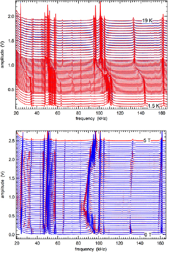
Figure 3. Segments of primary RUS spectra from Ba(Fe0.957Co0.043)2As2, crystal 1. Top: spectra collected in a field of 12.5 T (H//c) during heating (red) and subsequent cooling (blue). Bottom: spectra collected at 10 K with increasing (red) and decreasing field (blue). Individual spectra have been offset up the y -axis in proportion to the temperature or field at which they were collected. Resonance peaks which have no field or temperature dependence, particularly at low frequencies, are from the sample holder.
Download figure:
Standard image High-resolution imageIt was shown by Carpenter et al [20] that resonances of a thin crystal with the shape and dimensions used here are determined predominantly by different proportions of C66 and C11–C12, as defined with respect to the parent tetragonal crystal (Laue class 4/mmm). Those determined by C66 are easily identified by their strong temperature dependence through the ferroelastic transition at TS. Below TS there is an increase in the number of independent elastic constants to nine (Laue class mmm). However, a crystal which is cooled through the I4/mmm–Fmmm transition will contain approximately equal proportions of ferroelastic twins such that the average symmetry of the crystal as a whole will still be tetragonal. The resonances shown in figures 2 and 3 can therefore be considered as depending on combinations of C66, C11–C12 and C44, bearing in mind that these are averaged over all twin orientations.
4.1. C66: varying temperature at constant field
The temperature dependences of f 2 and Q−1 for selected peaks which, on the basis of large softening through the ferroelastic transition have been determined to be dependent predominantly on C66, are shown in figure 4. Full reversibility between heating and cooling is demonstrated in the close up view of a resonance peak with frequency near 140 kHz, as measured in a field of 12.5 T (figure 4(a)). The temperature interval of steep stiffening with falling temperature is marked also by variations in peak widths. These variations are shown quantitatively for a resonance mode near 330 kHz in different applied field strengths (figure 4(b)). The degree of softening in zero field reduces at 1 and 2.5 T, and becomes stiffening in fields of 5 T and above. Q−1 remains at low values through the temperature interval of the normal–superconducting transition in zero field but develops up to three successive Debye-like peaks when the transition is followed in an applied magnetic field.

Figure 4. Temperature dependence of f 2 and Q−1 at constant field for selected resonances depending predominantly on C66 (H//c). (a) Reversible evolution of an individual resonance peak during cooling (blue) and heating (red) in a constant field of 12.5 T. The spectra are stacked in proportion to the temperature at which they were collected. (b) Data for a resonance mode near 330 kHz show a small degree of softening with falling temperature in zero/low fields, without any anomaly in Q−1. This becomes stiffening at high fields, with the onset indicated by arrows, and the development of up to three peaks in Q−1. Reversibility is illustrated for f 2 data at 12.5 T: open circles = cooling, filled circles = heating. (c) f 2 data for a resonance near 25 kHz, which shows the largest degree of stiffening. Arrows indicate the temperatures at which the resistivity of the sample fell to 1% of its value in the normally conducting state for the cases of data collected in zero field and in a 12.5 T field. (d) Values of f 2 at 1.5 K taken from (c) reveal a parabolic dependence on field strength: the curve fit to the data is f 2 = 591 + 3.8(µoH)2.
Download figure:
Standard image High-resolution imageThe extent of stiffening varies between resonances but the greatest increase, by up to ~200%, occurs for a resonance near 25 kHz (figure 4(c)). The increased stiffness at 1.5 K scales with applied field as f 2  (µoH)2 (figure 4(d)).
4.2. C66: varying field at constant temperature
Details of the field dependence at 11 K of a resonance peak with frequency near 90 kHz are illustrated in figure 5(a). This mode is determined predominantly by C66 and, in addition to having changes in frequency and peak widths, reveals the clear hysteresis between increasing and decreasing field.
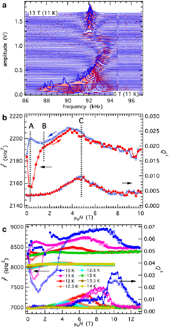
Figure 5. Field dependence of f 2 and Q−1 as a function of applied field at constant temperature for selected resonances depending predominantly on C66 (H//c). (a) Primary spectra stacked in proportion to the applied field, showing irreversible changes between increasing (red) and decreasing (blue) field. (b) Example of a resonance with frequency near 46 kHz, as measured at 12.3 K, showing three clear anomalies. A marks a minimum in f 2 at low fields in the sequence of increasing field strength, B marks the field at which there is a change from irreversible evolution to reversible evolution and C marks the Debye-like peak in Q−1 which accompanies a change of gradient in f 2. (c) More comprehensive data set for the resonance near 90 kHz, showing irreversibility between increasing (filled symbols) and decreasing field (open symbols) at 10, 11, 12 K. The fields at which irreversibility and broad peaks in Q−1 occur reduce with increasing temperature. (A small offset in the zero field frequencies between data collected to 10 T and data collected to 12.5 T is due to a change in ferroelastic twin configurations which occurred as a consequence of heating and cooling through the ferroelastic transition temperature in the interval between collecting the two data sets.)
Download figure:
Standard image High-resolution imageFigure 5(b) shows f 2 and Q−1 data obtained at 12.3 K for a resonance with frequency near 46 kHz. Specific features of the data are indicated by labels A, B and C. A marks the field at which a minimum in f 2 occurs at low values of µoH when the field is being ramped up. The loci of equivalent points at other temperatures are referred to below as 'H of low field anomaly, constant T'. The field at which the change from irreversible to reversible evolution occurs is labeled B and the loci of such points are referred to below as 'Hirr, constant T'. C marks the field at which there is a Debye-like peak in Q−1 and a change in the trend of f 2. This is referred to below as 'Q−1 peak, constant T'.
Figure 5(c) contains a compilation of f 2 and Q−1 data for the resonance with frequency near 90 kHz measured at temperatures between 10 and 14 K. It shows that the peak in Q−1 reduces in magnitude as temperature is increased and disappears altogether by 14 K. The amount of stiffening with reducing field associated with the loss peak diminishes at progressively higher temperatures, also disappearing by 14 K. Finally, the field at which the peak evolution changes from reversible to irreversible also reduces with increasing temperature.
Variations of f 2 and Q−1 below the limit of reversibility become more complex at progressively lower temperatures, as illustrated by an additional data set given in figure A1 for the resonance peak with frequency near 330 kHz.
4.3. C66: correlations between varying field and varying temperature
Values of the temperature and field at which the first loss peak with falling temperature under the condition of constant field (figure 4(b)) coincide with those for the single, broader acoustic loss peak observed when varying field at constant temperature (figure 5(c)). Values of the field at which the change from reversible to irreversible behaviour occurs correlate with field and temperature values for the second loss peak observed with falling temperature at constant field.
4.4. C11–C12 and C44
Some resonances of the sample showed no overt dependence on temperature through TS, TN and Tc. The peak with frequency near 175 kHz in figure 2 is an example of this for zero field and has been assigned to a primary dependence on C11–C12. Variations of f 2 and Q−1 for this resonance mode as a function of field at different temperatures are featureless up to 8 T, apart from a slight trend of increasing Q−1, as seen in figure 6. Resonances attributed to shearing controlled by C44 at higher temperatures [20] were too weak to allow them to be followed as a function of changing field.

Figure 6. Variations of f 2 and Q−1 with increasing and decreasing field at different temperatures for a resonance peak with frequency near 175 kHz. The f 2 data are featureless in the intervals of temperature and applied field where significant anomalies are present in data attributed to the variations of C66. There is only a slight increase in Q−1 with increasing field. This pattern is attributed to the variation of C11–C12.
Download figure:
Standard image High-resolution image4.5. Acoustic loss
In the interests of brevity, details of a formal analysis of the loss peaks are given in section A.2 and only fits to the data are shown in figure 7(a). Values of Ea/R extracted from the fitting, where Ea is the activation energy, R is the gas constant and Arrhenius thermal activation has been assumed (equation (A.1)), fall in the range ~250–600 K for the first peak, ~200–350 K for the second peak and ~100–200 K for the third peak (table A1). There are correlations with field strength and frequency but the strongest correlation is with temperature, such that the overall pattern is of a succession of anelastic pinning/freezing events with progressively smaller activation energy barriers as temperature reduces. Separate Arrhenius treatment of the frequency-temperature dependence of peak 1 with an external field of 7.5 T (figures 7(b) and (c)) gives Ea/R = 353 ± 3 K. f o values fall in the range 1015–1027 Hz, which is rather large to be physically realistic. Smaller values would be obtained for Vogel–Fulcher behaviour (equation (A.9)), but the frequency range is too narrow to allow this to be tested.

Figure 7. Kinetic analysis of acoustic loss. (a) and (b) Pink curves represent fits to individual loss peaks according to an Arrhenius description (Ea/R ⩾ ~370 K (peak 1), ⩾230 K (peak 2), ⩾125 K (peak 3), as set out in the appendix. Vertical dashed lines mark temperatures where the resistivity was 1% or 95% of that of the normal phase, ρn (see figure A4). Vertical dotted lines are the onset and extrapolated temperatures for the development of a diamagnetic moment (as illustrated in figure A5(a)). Data for f 2 in (b) have been multiplied by arbitrary scaling factors so that they can be compared on the same graph with data for the resonance near 25 kHz. (c) An Arrhenius plot of data from peak 1 in (b), where Tmax is the temperature at which the peak has a maximum value of Q−1. A straight line fit to the data has intercept and slope: lnf o = 43.0 ± 0.2, Ea/R = 353 ± 3 K.
Download figure:
Standard image High-resolution image5. Analysis
Variations in elastic constants associated with phase transitions arise as a consequence of coupling between strain and the driving order parameter(s). Here, anomalies in the temperature and field dependence of f 2 data that are clearly associated with the normal–superconducting transition appear to be restricted to resonances determined by C66. This indicates that the most significant strain component is e6. In the following analysis, focus is on strain coupling with the scalar driving order parameter, QSC, and on correlations with changes in heat capacity, electrical conductivity and magnetism for which details are given in the appendix.
5.1. Correlation with spontaneous strain
High resolution thermal expansion data for a crystal with composition Ba(Fe0.945Co0.055)2As2 are reproduced from Meingast et al [29] in figure 8(a). They reveal the overall pattern of strain variations which accompany the structural, magnetic and superconducting transitions. Changes of the a and c lattice parameters give strains Δa/a and Δc/c of up to ~0.0001 below TS ≈ 41 K, implying only very small changes in components e1 and e3 of the spontaneous strain tensor defined with respect to a parent tetragonal structure. By way of contrast, the value of e6, obtained by detwinning the crystal with an externally applied shear stress, increases to a maximum of ~0.0008 (figure 8(a), and see details in section A.3). The evolution of e6 can be understood in terms of its bilinear coupling with QE, λe6QE, though the tail above TS is due to the applied shear stress. The coefficient, λ, specifies the strength of coupling. There are no obvious deviations near TN (~29 K for the Co content of 0.055), implying that coupling of strains with the magnetic order parameter is very weak/absent.

Figure 8. Strain variations accompanying low temperature transitions in Ba(Fe1−xCox)2As2. (a) Linear expansion, Δl/l, volume strain and shear strain e6 for a crystal with x = 0.055 [29] all display small changes below TS, followed by a reversal in the direction of change below Tc. Dashed lines are baselines for the parent tetragonal structure, as described by equation (A.7) with saturation temperatures Θs = 80, 127, 115 K for Δa/a, Δc/c, ΔV/V. No anomalies are seen near TN. (b) The evolution of linear strain e1,SC defined with respect to the parent orthorhombic (normally conducting) phase of a crystal with x = 0.043 conforms to a second order transition below Tc = 12.5 K, as indicated by the smooth curve, which is a fit of equation (1) (Θso = 10.6 K). Changes in e6 below Tc are an order of magnitude larger but scale with temperature in essentially the same way.
Download figure:
Standard image High-resolution imageAn obvious and discrete reversal of all the trends in figure 8(a) occurs below Tc ≈ 22 K, consistent with an effective coupling of e1, e3 and e6 with QSC. This is expected to be of the form λei,SC , where ei,SC (i = 1, 3, 6) are components of the spontaneous strain defined with respect to the parent (normally conducting) orthorhombic crystal.
A formal analysis of less complete thermal expansion data for crystals from the same batch as used for RUS is given in section A.2 and the key results are shown in figure 8(b). The linear strain e1,SC has a temperature dependence which is consistent with a second order transition as
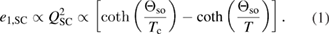
Following Salje et al [37], Θso is the order parameter saturation temperature. Figure 8(b) shows that changes in e6,SC are an order of magnitude larger than for e1,SC (up to ~8 × 10⁻⁵ instead of ~5 × 10⁻⁶), but follow the same trend, consistent with the expected relationships e1,SC ( e3,SC)
  e6,SC
e6,SC 
 .
.
The observed stepwise softening of C66, C11 and C33 through Tc in zero field (figure 4(b) and [16, 18, 19]) is typical of classical strain/order parameter coupling due to terms of the form λeQ2 at a second order transition (e.g. [38–40]). A step, with magnitude expected to scale with λ2, occurs between more or less constant values above and below Tc.
The pattern of slight elastic softening shown by C66 at 0, 1, 2.5 T, without overt changes in acoustic loss, becomes a pattern of stiffening at 5, 7.5, 12.5 T accompanied by successive peaks in Q−1 (figures 4(b) and 7(a)). The overall Debye-like form of this is typical for freezing or pinning processes of defects coupled with strain [41]. In this case the relevant strain must again be e6. Elastic stiffening has also been observed below the superconducting transition in cuprates, but the increases in elastic constants were orders of magnitude smaller than seen here and were accompanied by only a single loss peak [42].
5.2. Correlation of C66 with heat capacity, electrical resistivity and magnetism in zero field
Figure 9 contains a comparison of elastic softening in zero field, as expressed by variations of f 2 and Q−1 for selected resonances which depend predominantly on C66, with particular temperatures extracted from the measurements of heat capacity, electrical conductivity and magnetism that are set out in the appendix.
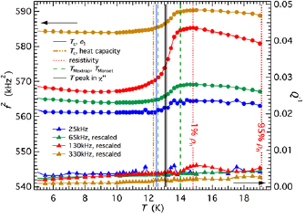
Figure 9. f 2 and Q−1 data from selected resonances which depend predominantly on C66 with slightly differing contributions of C11–C12 in spectra collected as a function of temperature in zero field. f 2 values have been multiplied by arbitrary scaling factors so that different resonances can be shown together. Vertical lines are different measures of the normal-superconducting transition temperature. 'Tc, e1' is the transition temperature estimated from the data for e1 in figure 8(b). 'Tc, heat capacity' is the transition temperature estimated from the observation of an anomaly in the heat capacity (figure A3). '1% ρn' and '95% ρn' mark the temperatures at which the resistivity reduced to 1% and 95% of values obtained for the normally conducting state (figure A4). 'TMonset and TMextrap' are the onset and extrapolated temperatures for the development of a diamagnetic moment (figure A5(a)). 'T peak in χ''' marks the temperatures at which there are maxima in the imaginary component of the AC magnetic susceptibility (with a slight frequency dependence, figure A6(a)).
Download figure:
Standard image High-resolution imageA step in the heat capacity at ~12.3 K (figure A3) is consistent with a discrete second order transition. This value of Tc is not distinguishable from the value of Tc = 12.5 K deduced from the Landau description of e1 (figure 8(b)).
Variations of electrical resistivity through Tc are shown in figure A4 and the temperatures at which it falls to 95% and 1% of the value for the normally conducting state are listed in table A2. In zero field, these are 19.1 and 14.8 K, respectively. There is no elastic anomaly near 19.1 K, but the 1% limit coincides with the onset of softening ahead of Tc (figure 9).
Two particular temperatures have been extracted from the variations of DC moment as a function of temperature shown in figures A5(a) and (b). The onset of a measurable diamagnetic moment in a field of 0.002 T, TMonset, is 14.0 K, which falls just ahead of the steepest segment of the softening trends in figure 9. Extrapolation of the linear segment of the increasing diamagnetic moment with falling temperature back to zero, TMextrap, gives 12.6 K, which is within experimental uncertainty of Tc determined from measurements of strain and heat capacity.
A steep change in the real part of AC magnetic moment, χ', and the accompanying peak in the imaginary part, χ'', are illustrated for selected frequencies and field strengths in figure A6. The peak in χ'' measured in a field of 0.002 T occurs at a temperature which is very slightly dependent on frequency (~13.0 K at 10 Hz, ~13.15 K at 10 kHz) and coincides with the midpoint of the steep elastic softening trend in figure 9.
In summary, measurements of bulk properties, ie spontaneous strain, heat capacity and DC moment, show that the normal—superconducting transition occurs at ~12.5 K. This is just below the temperature interval in which steep elastic softening of C66 occurs. The electrical conductivity measurements show the onset of superconductivity as occurring ahead of transformation in the bulk. AC magnetic anomalies correlate closely with the steepest part of the elastic softening.
5.3. Correlation of C66 with heat capacity, electrical resistivity and magnetism in applied magnetic field
Values of temperature and field for the peaks in Q−1 and initial breaks in slope of f 2 (ie of C66) illustrated in figures 4, 5, 7 and A1, together with additional data given in table A1, are combined in figure 10(a). Whether obtained in sequences of varying temperature at constant field or varying field at constant temperature, the data produce three clearly defined trends. With falling temperature at high fields, the first trend is for a peak in Q−1 (peak 1 in figure 7(a), C in figure 5(b)) accompanied by elastic stiffening characteristic of a Debye-like anelastic freezing process. The second trend is defined by the second acoustic loss peak seen with falling temperature (peak 2 in figure 7(a)) and the field, Hirr, at which a change from reversible to irreversible evolution of f 2 occurs (B in figure 5(b)). The third trend is at low fields and is given by the locus of the minimum in f 2 observed with increasing field strength at constant temperature below Tc (A in figure 5(b)). Peak 3 of Q−1 in figure 7(a) was only observed at the highest field strength.
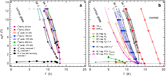
Figure 10. Correlation of elastic and anelastic properties with other properties of the superconducting phase. (a) Anomalies observed in RUS data collected by varying temperature at constant field (coloured symbols) and by varying field at constant temperature (black symbols) produce three well-defined boundaries. 'f 2 bend' marks the temperatures at which the first bend in f 2 occurs with falling temperature. 'Q−1 peak' marks the temperatures at which peaks in Q−1 occur. 'Q−1 peak, constant T' marks the field at which a peak in Q−1 occurs with varying field at constant temperature. 'Hirr, constant T' marks the temperature/field at which the trends of f 2 with increasing and decreasing field diverge. 'H of low field anomaly, constant T' marks the temperature/field where a minimum in f 2 occurs when varying field at constant temperature (see figure 5(b)). (b) The RUS data copied from (a) (grey symbols) correlate with magnetic and resistivity data (coloured symbols). '1% ρn' and 95% ρn' mark the temperatures at which the resistivity reduced to 1% and 95% of that for the normally conducting state. 'DC mag' signifies anomalies in magnetic properties measured with a DC field: Hirr is the limit of reversibility with increasing and decreasing field in hysteresis loops, as obtained in three different series of measurements. Hp and H2p refer to the fields at which the first and second peaks in moment occur with increasing field (see figures A5(c) and (d)). 'Hp × 7.4' is the value of Hp multiplied by a factor of 7.4 to take account of the difference in thickness between the thin crystal used for magnetic measurements and the thicker crystal used for RUS measurements. 'H for TMextrap' marks the field/temperature at which the magnetic moment measured as a function of temperature extrapolates to zero (see figure A5(a)). 'H for TMonset' marks the field/temperature at which the magnetic susceptibility first departs from a linear trend with falling temperature (see figure A5(a)). 'AC mag, peak in χ' marks the temperature/field at which a peak occurs in the imaginary part of the AC magnetic susceptibility measured at frequencies of 0.01, 0.1, 1, 10kHz. Dashed lines are polynomial fits to TMextrap and TMonset, allowing extrapolation to higher fields than were accessed experimentally.
Download figure:
Standard image High-resolution imageFigure 10(b) shows how the elastic anomalies correlate with changes in other properties as a function of temperature and field strength. The line for 95% resistivity is systematically ~4 K above the first elastic anomalies, while the line for 1% resistivity coincides with the trend of Debye-like freezing represented by peak 1 of Q−1 at field strengths of ~5 T and above. Below 2.5 T, the 1% line diverges and is ~2 K higher than the elastic anomalies in zero field.
AC magnetic data collected at frequencies of 0.01, 0.1, 1, 10 kHz in DC fields of 1, 2.5, 5, 7.5, 10 T all have a peak in the imaginary part of the susceptibility, χ'', accompanied by a steep change in the real part, χ', with a strong dependence on frequency (figures A6(b) and (c)). A more complete analysis of these is given in section A.7 and is discussed below. Here it is necessary only to note that this pattern is explained in the literature as being due to glassy freezing of vortices [43–45] and that the temperature-field locus of the anomalies overlaps at the high frequency end with the locus of acoustic loss peak 2 and Hirr of f 2 from the RUS data. The RUS data are for frequencies in the range ~25–350 kHz.
Values of TMextrap and TMonset from DC measurements of magnetic moment are listed in table A3 and define two curves in figure 10(b). At the lowest measuring field (0.002 T), TMonset is ~1 K above the temperature at which anomalies in the AC response occur but, at fields of 1 T and above, the curve for TMonset lies parallel to and just below the curves for AC magnetic loss. On this basis, TMonset appears to correspond to a static (zero frequency) measurement of the same process being sampled in the AC measurements and the acoustic loss process detected in the RUS measurements. The curve for TMextrap occurs systematically ~1–2 K below the curve for TMonset and does not obviously correlate with any changes in elastic properties, apart from its extrapolation passing close to acoustic loss peak 3 at 12.5 T.
Magnetic hysteresis loops measured to ±6.7 T show the fishtail pattern characteristic of an unconventional superconductor (figure A5(c)). Three specific points which occur with increasing field in these loops are Hp, the field at which there a maximum in moment occurs during the first increase from zero, H2p, the field at which there is a rounded maximum in the moment and Hirr, the field at which the change from reversible to irreversible evolution occurs. Hp is understood to be the field at which vortices nucleated at the surface of a crystal reach its centre [46] and H2p has been explained in terms of a change in pinning properties of the vortices (e.g. [47]). Irregular variations of f 2 evident at low fields below the interval of vortex freezing include minima (A in figure 5(b)) which are in the same part of the phase diagram as H2p and Hp, though the correlation is not exact (figure 10(b)). Values of Hirr for the evolution of moment in the hysteresis loops differed between two different series of measurements (see section A.6 below), but nearly all fall between TMonset and TMextrap. This is just below the temperature range in which the loss process indicated by the AC magnetism and RUS data occurs.
6. Discussion
The most general result from the observation of systematic acoustic anomalies associated with superconductivity in Ba(Fe0.957Co0.043)2As2 is that there is significant coupling of strain with the normal-superconducting transition in zero field, the development of vortices in an applied field and the dynamics of vortex motion when temperature and field are changed. Anomalies in the elastic properties at low temperatures relate to the evolution of C66, which implies that the important strain effects relate predominantly to e6. The implications of these can be explored in detail here because systematic measurements were made of other properties of crystals from the same original batch.
6.1. Order parameter coupling
The most fundamental consequence of coupling of order parameters with strain is suppression of fluctuations and promotion of mean field behaviour due to the long ranging nature of strain fields. Data for heat capacity, evolution of the spontaneous strain and softening of C66 are all consistent with a description of the normal-superconducting transition in zero field as being a classical second order phase transition with coupling of the form λe6 .
.
If there is coupling between strain and order parameters of the form λe6 and λe6QE, there must also be coupling of the order parameters with the form λ
 QE via the common strain. If there is also coupling of QE with QM it follows that all three order parameters are coupled, so defining the existence of multiferroic superconductivity in a single phase. In the case of Ba(Fe0.957Co0.043)2As2, the significant coupling is between QSC and QM and all three order parameters vary together. By way of contrast, YBCO does not belong to this class, in effect, because the tetragonal–orthorhombic transition occurs hundreds of degrees above Tc [48, 49] and antiferromagnetic ordering also appears to be quite separate (e.g. [50]).
More generally, linear-quadratic coupling occurs when one of the instabilities is proper or pseudoproper ferroelastic and leads to distinctive phase diagram topologies [51, 52], which must be a significant factor in the phenomenological richness of the behaviour of pnictides with respect to changes in composition, temperature, magnetic field, pressure, stress, etc.
6.2. Strain contrast associated with vortices
The existence of a contrast in the shear strain e6 between normal and superconducting states of Ba(Fe0.957Co0.043)2As2 means that there must also be shear strain contrast between vortex cores and the superconducting matrix. It follows inevitably that interactions between vortices and of vortices with their surrounds will be mediated by long ranging strain fields, in much the same manner as is evident in the way that twin walls in ferroelastic materials interact with each other over lengths scales of up to ~0.1 µm (see, for example, chapter 7 of [53]). Relatively stiff vortices in a relatively soft superconducting matrix would lead to an increase in overall stiffness with increasing field simply because of the expected increase in the density of vortices. However, the strain fields around each vortex will give rise to additional interactions between them. Strong repulsive forces arising from unfavourable overlapping of these would give an additional increase in resistance to specific orientations of shear stress and are likely to be a significant factor in the steep increases in stiffness evident in figure 4. Changes in elastic stiffness will depend on the orientation of the vortices which, in turn, depends on the orientation of the magnetic field. In the present study, the vortices will have been aligned parallel to [0 0 1] of the parent tetragonal structure and the observed changes are in elastic constants are for C66. This means that the relevant repulsive forces between vortices will have been within the (0 0 1) plane, ie perpendicular to their lengths.
Whatever microscopic model is developed to account for the added stiffness per vortex, a linear dependence on field strength is not expected because reversing the sign of the field would not change their density and distribution. Instead, the maximum amount of stiffening, i.e. for the fully frozen state at 1.5 K, displays a parabolic dependence on applied field (figure 3(d)), as previously reported for YBCO [14].
6.3. Vortex liquid–vortex glass transition
The complete analysis of AC magnetic data in section A.7 is consistent with views from the literature that the Debye-like anomalies in χ' and χ'' in an applied magnetic field are due to freezing of vortices. Analysis based on Vogel–Fulcher dynamics (equation (A.9)) and the Havrilian–Negami equation (equation (A.10)) provide a reasonable description of the frequency dependence for a process which involves a small spread of relaxation times. In an RUS experiment the range of accessible frequencies corresponds to only ~1 log unit but data for Q−1 of peak 2 measured at 10 and 12.5 T fall on extrapolations to data for χ'' plotted in Arrhenius form (figure 11). This shows that the same liquid—glass transition is being detected and demonstrates that the vortices couple significantly with strain.

Figure 11. Arrhenius plot of the relationship between measuring frequency, f , and the temperature, Tm, at which loss peaks occur in AC magnetic data and elasticity data from RUS. The RUS data plot on or close to extrapolations of lines fit to the AC magnetic data.
Download figure:
Standard image High-resolution imageValues of field for DC measurements of the onset of irreversibility in hysteresis loops, Hirr in figures A8 and 10(b), and of temperature for the first appearance of a diamagnetic moment, TMonset, fall just below the dynamic magnetic measurements, consistent with their marking the static limit of the freezing process. With respect to elasticity, the limit of reversibility in variations of f 2 with changing field at constant temperature, Hirr in figure 10(a), corresponds to the freezing point, as measured at frequencies in the vicinity of ~100 kHz.
Values of ~200–300 K (~17–26 meV) for the activation energy estimated from Arrhenius treatment of acoustic loss peak 2 (table A1) compare with ~10–70 K (~1–6 meV) from Vogel–Fulcher analysis of the AC magnetic loss peaks (section A.7). These are comparable with a previous determination of 120 ± 20 K for vortex freezing in Ba(Fe0.93Rh0.07)2As2 [54].
6.4. Vortex pinning mechanisms and the elastic properties of vortex glass
The structural landscape through which vortices move in Ba(Fe1−xCox)2As2 is believed to be homogeneous in the sense that antiferromagnetism and superconductivity coexist without phase separation [3–8, 55]. However, while it may be single phase, local strain heterogeneities must exist on a unit cell scale due to the size difference of Co substituting for Fe [56]. The existence of local electronic inhomogeneity has already been discussed in the context of other measurements, including, for example, heat capacity and NMR line broadening [57–59], as well as magnetic dependence of critical current density [60]. This local strain heterogeneity is likely to influence the effective viscosity experienced by mobile vortices and the strength of pinning processes within the glass state.
Activation energies from Arrhenius and Vogel–Fulcher treatments of the Q−1 and AC magnetic data (figure 7 and sections A.2 and A.7) all fall in the range ~50–600 K, which overlaps with the range of values estimated for the pinning of ferroelastic twin walls (400–750 K) at higher temperatures [20]. This is also the same energy scale as reported for resistivity and acoustic attenuation in other superconductors (e.g. [61]), including ~200 K for polaron-like conductivity in BaFe2As2 [62] and ~850 K for anelastic loss in YBCO [63]. It appears that the pinning/freezing processes are controlled by essentially the same activation barriers as the mobility of polarons, for which coupling with a local strain cloud provides the most likely constraint. The magnitude of the activation energy estimated from Q−1 peaks 1–3 reduces with falling temperature (table A1), showing that there is a sequence of pinning/freezing mechanisms associated with progressively lower pinning potentials.
RUS data collected as a function of temperature at constant field are relatively featureless below the vortex liquid–vortex glass transition and the evolution of f 2 for all resonances is fully reversible (figure 4). This implies that a fixed density of vortices is established in the liquid state and that their configuration does not then change in response to increasing or decreasing temperature. Increases in the height of the broad loss peak at progressively higher fields (figure 4(c)) can be understood simply in terms of the increase in the number of vortices present.
Significant variations in elastic properties occur when the field is increased at constant temperature below their freezing point, due to changes in both density and configuration. Hp from hysteresis loops (figure A5) can be understood as marking the field at which vortices nucleated at the surface of a crystal first penetrate to its centre [46]. Anomalies in f 2 do not correlate exactly with these (figure 10(b)), but are sufficiently close to be understandable on the same basis. With increasing field, the density of vortices will increase but their distribution will be fixed by pinning points. At sufficiently high fields the glass transition point is exceeded and the vortices become mobile, but hysteresis in the elastic properties of the crystal as a whole below Hirr implies that they acquire a different configuration on refreezing.
H2p has been interpreted as a change in pinning properties of the vortices [47] but there does not appear to be any equivalent anomaly in elastic or anelastic properties associated with this (figure 10(b)). The low stress experienced within a resonating crystal during an RUS experiment [64, 65] is presumably well below the critical stress that would be needed to unpin the vortices.
6.5. Elastic properties of vortex liquid: superconductivity along ferroelastic twin walls?
There is, perhaps, a slight decrease in the rate of elastic stiffening with falling temperature which correlates with the 95% resistivity limit (figures 7(a) and (b)), but there is no other obvious anomaly at this point. If so, the softening mechanism is likely to be analogous to the effect of polar nanoregions in relaxor ferroelectrics such as PbMg1/3Nb2/3O3 where acoustic phonons interact with a dynamical local domain microstructure (e.g. [66]). Local dynamical regions of superconductivity would generate locally fluctuating strain fields which, in turn, would interact with acoustic phonons to give the slight softening.
Evidence from strain, heat capacity and AC magnetism in zero field is for a discrete phase transition ~2 K below the temperature at which resistivity reduces to 1% of its value in the normally conducting state (figure 8). This value is generally taken as marking the onset of superconductivity but it is not accompanied by any elastic anomaly beyond a slight acceleration of the softening trend. On the other hand, the line for 1% resistivity at high fields correlates closely with the Debye-like combination of elastic softening and acoustic loss referred to in figures 7 and 10 as peak 1. This is ~2 K ahead of the interval of vortex freezing, and data of Ni et al [30] have shown the same discrepancy systematically in other underdoped crystals. The onset of superconductivity and the occurrence of some pinning/freezing process responsible for the acoustic loss are within what is expected to be the stability field of vortex liquid. However, changes in magnetic properties which would indicate superconductivity throughout the bulk of the crystal only appear at lower temperatures and two obvious explanations are that an initial reduction in resistance takes place in surface layers only or that some percolative superconducting pathways develop through the crystal.
Given that the microstructure of Co-doped orthorhombic crystals in the underdoped range is of two sets of orthogonal twin walls, with a tweed like pattern on a scale of <2 µm for individual domains [67], an interesting possibility is that the twin walls could provide the percolating pathways of superconductivity. This would be consistent with previous observations of enhanced superfluid density on twin walls below Tc [68, 69]. The associated loss peak would be understandable in terms of pinning or freezing of vortices close to the superconducting twin walls.
6.6. Strain-mediation of interactions between vortices and ferroelastic twin walls
The lesson from ferroelastic materials with more than one order parameter is that twin walls can have structures and properties which are distinct from both the parent phase and the matrix in which they lie. A perovskite example of this is the development of ferrielectric dipoles at the ferroelastic twin walls in CaTiO3 [70]. Linear-quadratic coupling generates new possibilities for a variety of exotic domain walls [71]. In the present case, there must be strain-mediated interactions between vortices and ferroelastic twin walls via all of the common strains e1, e3 and e6. The evidence from a crystal with x = 0.055 (figure 8(a)) is that, like e6, the sign of linear strains which couple with the ferroelastic order parameter is the reverse of the linear strains with couple with the order parameter for superconductivity. Superconductivity should therefore be favoured in regions of the crystal where these strains are smallest, ie within the ferroelastic twin walls. Vortices will be favoured in regions where the ferroelastic strain is large, ie away from the ferroelastic twin walls. This strain argument is consistent also with the fact that vortices in Ba(Fe1−xCox)2As2 are repelled from the twin walls [69] and that the twin walls influence the vortex glass transition itself at low fields [72].
In the context of ferroelastic properties, YBCO again provides a contrast in that vortices have been observed to decorate the twin walls [73–75] rather than being repelled from them. The implication is that the flux density will be reduced along the walls in comparison with the bulk and, according to the arguments presented here, this is likely to be a consequence of favourable strain coupling between the walls and the vortices. FeSe is more like Ba(Fe1−xCox)2As2 than YBCO in that ferroelasticity and superconductivity are coupled. However, vortices accumulate on the twin walls and superconductivity along the walls is degraded [76].
This aspect of the pnictides remains to be fully explored but it must be expected that the superconducting properties of the ferroelastic twin walls could be engineered by choices of chemistry, temperature and field. With respect to the possibilities for domain wall engineering, the interesting question is whether it might be possible to produce a wide field of stability for a pnictide with 2D superconductivity on the twin walls.
6.7. H–T phase diagram
In combination, the elasticity and magnetism data in figure 10(b) define two expected phase boundaries. Firstly, there is the onset of changes in resistivity. The line marking 90 or 95% of normal resistivity has previously been taken as an estimate for Hc2, (e.g. [60, 77–80]). When measured on the same crystal, values of Hc2 defined in terms of resistivity do not necessarily coincide with values defined in terms of magnetic susceptibility (e.g. [30, 78]). If this determination of Hc2 is correct, condensation of the mixed phase of mobile vortices in a superconducting matrix (vortex liquid) takes place between 5 and 10 K above the temperature at which the vortex glass transition occurs, as also reported by Shen et al [77] for a crystal with x = 0.06. The 95% line is interpreted here as representing a diffuse boundary between normally conducting behaviour and the development of dynamical regions, with local superconductivity and/or mobile vortices, which couple with acoustic phonons sufficiently to cause an onset of elastic softening. Interpretation of the second boundary due to the vortex liquid–vortex glass transition, as defined by frequency dependent magnetic and acoustic loss peaks, is more secure. It is closely followed by changes in DC magnetic properties that mark the static limit of the freezing process.
A third boundary, seen in both magnetic and elastic properties at low fields within the stability field of the vortex glass, is interpreted as defining the limit with increasing field where vortices nucleated at the surface of the crystal penetrate through to its centre. However, the exact location of this boundary would be expected to vary with the thickness of the crystal and adjustment by a factor of 7.4 in the position of Hp in figure 10(b) has been made to allow for the difference in thickness of the crystals used for the magnetic and RUS measurements.
The physical origin of the fourth boundary, marked by the overlap of acoustic loss peak 1 and the line for 1% resistivity, is less obvious as it appears to be located in what would be expected to be the stability field for a vortex liquid. The divergence of these two lines below ~2 T suggests that the acoustic loss is related to the presence of vortices. As discussed above, the most interesting possibility is that it relates to the development of percolative pathways for superconductivity along ferroelastic twin walls. In order to test this, it will be necessary to investigate the elastic properties of pnictide crystals which remain tetragonal through the normal–superconducting transition and would not, therefore, contain ferroelastic twins. Otherwise, the superconducting pathway could be in the surface layers of the crystal.
7. Conclusions
Strain is well known to have a permeating influence on phase transitions. Classic effects include suppression of fluctuations, promotion of mean field behaviour, coupling between multiple order parameters, control of the configuration of transition-related microstructures and pinning of mobile microstructures by defects. The most general conclusion from the present study is that intrinsic and extrinsic strain coupling effects have a similar bearing on the superconducting properties of single crystal Ba(Fe0.957Co0.043)2As2. Considerations of multiferroic superconductors should lead to new possibilities for domain wall engineering involving control of resistivity, magnetism, ferroelasticity and microstructure through coupling of the separate order parameters at a nano scale. More specific conclusions from combining measurements of elastic and anelastic properties with measurements of spontaneous strain, resistivity, heat capacity, DC magnetism and AC magnetism are:
- 1.Softening due to classical strain/order parameter coupling occurs at the normal–superconducting transition in zero field. Evolution of the spontaneous strain is consistent with a standard mean field representation of a second order phase transition.
- 2.With increasing field, any softening due to strain/order parameter coupling is overwhelmed by Debye-like elastic stiffening and acoustic loss related to the vortex liquid–vortex glass transition. The substantial strain relaxation effects which are associated with the freezing process indicate that the dominant process is likely to be interaction of vortices with strain heterogeneities in the host crystal structure.
- 3.The vortex liquid–vortex glass transition is preceded by an additional pinning or freezing process which correlates exactly with the field and temperature at which resistivity reduces to 1% of the value for the normally conducting phase. The underlying mechanism has not been established but could be related to superconductivity becoming established in surface layers of the crystal or as percolating pathways along ferroelastic twin walls.
- 4.If there is strain contrast between normal and superconducting phases, there must be a similar strain contrast between the cores of vortices and their surrounding superconducting matrix. Interactions between individual vortices will be enhanced by overlapping strain fields and will contribute to the substantial stiffening associated with their immobilisation.
- 5.Interaction between vortices and ferroelastic twin walls must occur via their associated strain fields. This interaction appears to be unfavourable, which would account for the repulsion of vortices from the twin walls and are likely to be a significant factor in enhancing superconductivity within the twin walls.
Acknowledgments
Measurements of AC magnetic properties, electrical resistivity and heat capacity were carried out in the Advanced Materials Characterisation Suite, funded by EPSRC Strategic Equipment Grant EP/M000524/1, PM acknowledges funding from the Winton Programme for the Physics of Sustainability. Tony Dennis is thanked for help with collection of the DC magnetic data. Funding for the work was provided through EPSRC grant no. EP/I036079/1.
Appendix. Additional sample characterisation
A.1. Additional elasticity data
Figure A1 shows data for the field dependence of f 2 and Q−1 at nine different temperatures from a resonance peak near 330 kHz, which predominantly reflects the variation of C66. The variations become increasingly hysteretic as temperature is reduced.

Figure A1. Hysteresis effects and irregular variations at low fields seen in data collected as a function of field (H//c) at different temperatures for a resonance which depends predominantly on C66, with frequency in the vicinity of 330 kHz. Filled circles = f 2 with increasing field, open circles = f 2 with subsequent decreasing field, filled triangles = Q−1 with increasing field, open triangles = Q−1 with decreasing field.
Download figure:
Standard image High-resolution imageA.2. Analysis of acoustic loss peaks
Peaks in Q−1 and the accompanying increases in f 2 with falling temperature appear to be consistent with Debye-like loss processes associated with freezing of defects. On this basis, the temperature dependence of the loss can be described by [81–84]
where the maximum value of Q−1,  , occurs at temperature Tmax, Ea is an activation energy conforming to equation (A.8), below, and r2(γ) is a width parameter. Values of r2(γ) specify a spread of relaxation times, as set out in tables 4-2 of Nowick and Berry [41]. It is unity for a single relaxation time (γ = 0), and increases as the spread increases.
Table A1 contains parameters obtained by fitting equation (A.1) to a selection of the acoustic loss peaks, as illustrated in figures 7(a) and (b). Values of Ea/R fall in the range ~250–600 K for the peak associated most closely with the normal-superconducting transition (peak 1), ~200–350 K for the peak associated with the vortex glass transition (peak 2) and ~100–200 K for peaks which fall at lower temperatures than these (peak 3). There are trends with external field and frequency but the dominant correlation is with values of Tmax such that loss peaks at the highest temperatures have the highest effective thermal barriers, while those at the lowest temperature have the lowest barriers. Variations of Q−1 for peak 1 at 7.5 T are sufficiently well constrained to give lnf o = 43.04 ± 0.24 (f o = 4.9 × 10¹⁸ Hz) and Ea/R = 353 ± 3 K from a conventional Arrhenius treatment (figures 7(b) and (c)). This compares with 596, 278 and 265 K (average 380 K) from fitting of the individual peaks at the three different frequencies. γ = 1 or 2, for which r2(γ) = 1.26 or 1.74 [41], would give values of Ea/R extracted from the individual peaks that are 26 and 74% higher, respectively, which would take them increasingly out of the range of the conventional Arrhenius result. Thus, if there is a spread of relaxation times associated with the acoustic loss mechanism at the normal-superconducting transition it is only small, which is consistent with the result from the Havrilian–Negami treatment of AC magnetic data for vortex freezing, below. Values of f o were obtained by inserting values of Ea/R into equation (A.8).
Table A1. Values of parameters obtained by fitting equation (A.1) to peaks in Q−1, as illustrated in figures 7(a) and (b).
| Peak no. | Frequency (kHz) | Field (T) | Qmax | Tmax (K) | Ea/R, γ = 0, r2(γ) = 1 | f o (Hz) | ln f o |
|---|---|---|---|---|---|---|---|
| 1 | 329.8 | 12.5 | 0.008 | 9.76 ± 0.02 | 374 ± 26 | 1.45 × 10²² | 51.02 |
| 2 | 338.6 | 12.5 | 0.011 | 7.20 ± 0.02 | 228 ± 17 | 1.92 × 10¹⁹ | 44.40 |
| 3 | 340.1 | 12.5 | 0.003 | 5.01 ± 0.02 | 125 ± 15 | 2.33 × 10¹⁶ | 37.69 |
| 1 | 329.4 | 10 | 0.006 | 11.02 ± 0.02 | 559 ± 41 | 3.53 × 1027 | 63.43 |
| 2 | 333.3 | 10 | 0.005 | 9.11 ± 0.05 | 210 ± 32 | 3.42 × 10¹⁵ | 35.77 |
| 3 | 342.6 | 10 | 0.005 | 7.74 ± 0.03 | 175 ± 17 | 2.26 × 10¹⁵ | 35.35 |
| 1 | 330.5 | 7.5 | 0.006 | 11.64 ± 0.02 | 596 ± 45 | 5.70 × 1027 | 63.91 |
| 1 | 135.0 | 7.5 | 0.009 | 11.31 ± 0.02 | 278 ± 16 | 6.39 × 10¹⁵ | 36.39 |
| 1 | 67.4 | 7.5 | 0.020 | 11.06 ± 0.02 | 265 ± 12 | 1.72 × 10¹⁵ | 35.08 |
| 2 | 69.1 | 7.5 | 0.009 | 9.74 ± 0.03 | 308 ± 33 | 3.74 × 10¹⁸ | 42.77 |
| 2 | 136.0 | 7.5 | 0.010 | 9.62 ± 0.04 | 325 ± 46 | 6.39 × 10¹⁹ | 45.60 |
A.3. Strain analysis
A formal treatment of selected spontaneous strains accompanying the phase transitions in Ba(Fe1−xCox)2As2 at compositions near x = 0.45 has been given elsewhere [20]. There are two non-symmetry breaking strains, e1 (=e2) and e3, and a symmetry breaking shear strain, e6. These are related to the structural/electronic order parameter, QE, as e6  QE and e1
  e3
e3 
 due to coupling terms of the form λe6QE, λe1
 and λe3
 . The equivalent coupling terms for a scalar order parameter due to the superconducting transition, QSC, are λe6,SC
 , λe1,SC
 and λe3,SC
 , so the contributions to e6, e1 and e3 below Tc, e6,SC, e1,SC, e3,SC, are expected to scale with
  .
.
The conventional way of determining variations of these strains with temperature would be from lattice parameter data obtained by diffraction methods. However, data can also be extracted from changes in the linear dimensions of a single crystal with respect to a reference state at a temperature above TS, according to
and
Δa/a and Δc/c are the relative length changes within and perpendicular to the (0 0 1) plane, respectively, of a twinned single crystal of the orthorhombic phase. (Δa/a)o, (Δc/c)o are relative length changes of the tetragonal parent crystal extrapolated to temperatures below TS. Changes in volume below TS can be taken as
The symmetry breaking shear strain, e6, due to the tetragonal–orthorhombic transition is given by
where a and b are lattice parameters of the orthorhombic structure. Linear thermal expansion data for both Δa/a and Δb/b can be obtained by applying a detwinning shear stress to the crystal [85]. Values of e6 are then given by
As shown in figure 4 of Böhmer et al [85] for a different 122 phase, this reveals the form of the lattice distortion below TS. The detwinning stress results in an additional contribution to e6, which appears as a tail stretching to higher temperatures.
Variations of linear strains and the volume strain just above and through Tc are given for a crystal with x = 0.055 in figure 8(a), based on primary data from Meingast et al [29]. Equivalent data are not available for crystals with x = 0.043, apart from the variations of Δa/a and e6 shown in figures A2(a) and (c), which were obtained using the techniques described in Böhmer et al [85] for a crystal taken from the same batch as used for the present study. In order to determine e1 due to the superconducting transition alone, e1,SC, values of (Δa/a)o, have been obtained by fitting the function
to data in the temperature interval immediately above Tc and extrapolating to lower temperatures (figure A2(a)). Resulting changes in e1,SC, which should scale with  , are shown in figure A2(b).

Figure A2. (a) Linear thermal expansion of a single crystal with composition Ba(Fe0.957Co0.043)2As2. The solid line is a fit of equation (A.7) to data between 13.6 and 20 K; Θso = 30 K. (b) Variations of e1,SC (red data points), calculated from the data shown in (a), and DC moment (in 0.002 T field, blue data points). The curve through the data for e1,SC is a fit of equation (1) with Θso = 10.6 K and Tc = 12.5 K. The straight line fit to the magnetic moments extrapolates to zero at 12.6 K. Both sets of data have a weak tail up to slightly higher temperatures. (c) Expanded view of the low temperature variation of e6, showing how the contribution associated with the normal-superconducting transition, e6,SC, is given by the difference between extrapolated values of the Landau solution for a second order ferroelastic transition and observed values below Tc.
Download figure:
Standard image High-resolution imageA fit of equation (1) to the data for e1,SC gives Tc = 12.5 ± ~0.1 K (figure 8(b)). The straight line fit to data for the DC magnetic moment measured at 0.002 T (section A.6, below) in the small temperature interval where they vary steeply extrapolates to zero at 12.6 ± ~0.1 K. Not only do both sets of data give the same value of Tc, but they also have a tail that extends up to between ~13.5 and ~14.0 K (figure A2(b)). Figure A2(c) shows the variation of e6 in the lowest temperature range, with a curve based on equation (A.1) fit to data in the interval 15–41 K and extrapolated down to 5 K. Values of shear strain due to the superconducting transition, e6,SC, have been taken as the difference between the extrapolation and measured values. Variations of e1,SC and e6,SC with temperature are shown together in figure 8(b).
The magnitudes of strains associated with the superconducting transition are substantially smaller than those associated with the ferroelastic transition. For, example, by coupling with the ferroelastic order parameter e1 reaches values of ~ −1.6 × 10⁻⁴ (at x = 0.047) and e6 reaches values of ~2.7 × 10⁻³ (at x = 0.045) [20]. Below the superconducting transition, the change in e1,SC for the crystal with x = 0.043 is up to ~6 × 10⁻⁶ (figure A2(b)) and the change in e6,SC for is up to ~ −7 × 10⁻⁵ (figure A2(c)). It follows that changes in elastic constants due to strain coupling are expected to be substantially smaller for the normal–superconducting transition than for the ferroelastic transition and that changes in C11, C12 and C33 associated with the superconductivity are expected to be substantially smaller than those associated with C66.
A.4. Heat capacity
The heat capacity of Crystal 2 was measured using the heat capacity option of a Quantum Design PPMS. Data collected in 0.1 K steps through the range 8–18 K from two separate runs are shown in figure A3. An arbitrary polynomial function has been fit to data in the higher temperature range to highlight the small anomaly in the vicinity of 12.5 K. The form of the anomaly is closely similar to that shown elsewhere for Ba(Fe1−xCox)2As2 crystals with ranges of composition between x = 0.038 and 0.14 [18, 28, 30, 86–88]. It is in the form of a small, rounded step, with a slight tail to higher temperatures, consistent with expectations for a second order phase transition. The step, ΔCp, shown at Tc ≈ 12.3 K is ~0.05 J mol−1 K−1. In the treatment of Ni et al [30], Tc was taken as the temperature at which the tail reached baseline values, as determined by comparing with data collected at 9 T, which would give a slightly higher value than the definition used here.

Figure A3. Heat capacity of crystal 2 at low temperatures, as measured in two separate experimental runs. Solid lines are curves fit to data in the range ~14–18 K in order to reveal the small anomaly associated with Tc, which is taken to be 12.3 K. The step at Tc, ΔCp, is ~0.05 J mol−1 K−1.
Download figure:
Standard image High-resolution imageA.5. Resistivity
Four electrical leads were attached to the surface of Crystal 2 for measurement of in-plane resistivity (ρ) using the Electrical Transport Option of a 14 T PPMS from Quantum Design, with an AC current of 1 mA at 18.1 Hz. The temperature sweep rate was 0.3 K min−1, with steps of 0.15 K during heating and cooling through the temperature interval 2–20 K. These measurements were repeated in successively increasing magnetic field strengths of 0, 0.002, 1, 2.5, 5, 7.5, 10 and 12.5 T applied perpendicular to the large faces of the crystal (H//c). Results are shown in figure A4, and the temperatures listed in table A2 were determined by drawing horizontal lines at values of ρ corresponding to 1, 10, 90 and 95% of the resistivity of the normal phase, ρn. The difference in temperature between 10% and 90% of ρn in zero field is 2.6 K and remains less than 3 K at all fields, consistent with results reported for a crystal with x = 0.1 by Yamamoto et al [60]. The zero-field value reported by Sefat et al [89] for a crystal also with x = 0.1 was 0.6 K.
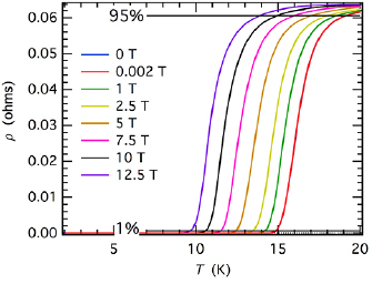
Figure A4. In plane resistivity, ρ, of crystal 2 measured in different magnetic field strengths (H//c). There were no differences between results for heating and cooling. Data collected in zero field and at 0.002 T overlap closely, and are not distinguishable on this scale. Horizontal lines mark 1% and 95% of the resistivity of the normal phase, ρn.
Download figure:
Standard image High-resolution imageTable A2. Temperatures for specific levels of resistivity, as determined from horizontal lines drawn across the resistivity curves in figure A4. ρn is the resistivity of the normally conducting state.
| Magnetic field strength (T) | T (K) at 1% ρn | T (K) at 10% ρn | T (K) at 90% ρn | T (K) at 95% ρn |
|---|---|---|---|---|
| 0 | 14.8 | 15.4 | 18.0 | 19.1 |
| 0.002 | 14.8 | 15.4 | 18.0 | 19.1 |
| 1 | 14.2 | 14.7 | 17.4 | 18.6 |
| 2.5 | 13.5 | 14.0 | 16.7 | 18.0 |
| 5 | 12.5 | 12.9 | 15.8 | 17.0 |
| 7.5 | 11.5 | 12.0 | 14.7 | 15.9 |
| 10 | 10.6 | 11.1 | 13.8 | 14.9 |
| 12.5 | 9.7 | 10.2 | 12.8 | 13.9 |
A.6. DC magnetism
Measurements of DC magnetic moment made on Crystal 2 over a wide temperature interval have been reported previously [20]. For the present study, a new set of measurements were made in a Quantum Design MPMS XL squid magnetometer with H//c. Cooling was in zero field followed by heating with the field on. The data shown in figure A5 are from heating sequences between 2 and 20 K in steps of 0.2 K at progressively higher fields (0, 0.002, 1, 2.5, 5, 7 T). These are shown as susceptibility, M/H, in figure A5(a) and were used to determine the two separate temperatures listed in table A3. The first is the temperature at which extrapolation of a linear segment of the variation of diamagnetic moment with temperature extrapolated to zero, TMextrap, and the second is the onset temperature for a diamagnetic response with falling temperature, TMonset. A measure of the sharpness of the transition at low fields is provided by the difference between the temperatures at which the values of M/H are 10 and 90% of that of the superconducting phase at low temperatures. Here this value is 0.8 K, which is comparable with 0.5 K reported by Marsik et al [3] for a crystal with x = 0.055.
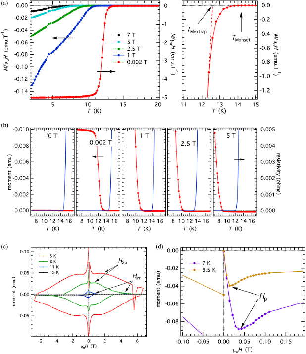
Figure A5. DC magnetism. (a) Magnetic susceptibility determined from crystal 2 in heating sequences from 2 to 20 K under progressively higher applied magnetic field. The anomalous response in the vicinity of 4 K is an artefact due to condensation of He gas to liquid in the instrument. Also shown is an illustration of how values of TMextrap and TMonset were defined. (b) Comparison of the temperature dependences of DC moment (red, left axis) and resistivity (blue, right axis) in the vicinity of Tc under the influence of external magnetic fields between 0 and 5 T (H//c). The label for 0 T is in inverted commas to signify that measurements were made simply with the magnet field switched off. (c) Hysteresis loops collected in the range +6.7 to −6.7 T, H//c (after Carpenter et al [20]). H2p represents the magnetic field strength of the second peak of each loop and Hirr represents the field at which the upper and lower portions of each loop converge. (d) Initial segments of hysteresis loops with sufficiently high resolution to allow determination of the field at which the maximum of the first peak, Hp, occurs on increasing field from zero.
Download figure:
Standard image High-resolution imageTable A3. Values of TMonset and TMextrap estimated from the DC magnetic data shown in figure A5(a).
| Magnetic field strength (T) | TMextrap (K) | TMonset (K) |
|---|---|---|
| 0.002 | 12.6 | 14.0 |
| 1 | 10.6 | 12.0 |
| 2.5 | 9.1 | 10.7 |
| 5 | 7.4 | 9.4 |
| 7 | 6.4 | 8.4 |
Variations of DC moment and resistivity in the vicinity of Tc are shown together in figure A5(b). Under the influence of external magnetic fields through the range 0.002–5 T there is a difference of ~2–3 K between the temperatures at which the resistivity tends to zero and the DC moment tends to its high temperature value, which is also close to zero.
Magnetic hysteresis loops (H//c) measured to ±6.7 T are reproduced from Carpenter et al [20] in figure A5(c). They show the typical fishtail pattern of an unconventional superconductor. M–H loops collected at higher temperatures were virtually indistinguishable from those collected at 15 K. A weakly ferromagnetic component is present and is attributed here to local moments rather than the presence of a ferromagnetic impurity phase. Values of H2p, the field at which the second peak occurs, and of Hirr, the field at which the top and bottom segments of each loop merge on increasing or decreasing field, are listed in table A4. Crystal 2 was used again for further hysteresis measurements at 7 and 9.5 K, with a focus on the initial magnetization using field steps of 0.0071 T in order to obtain estimates for the position of the first peak, Hp, as shown in figure A5(d). Values of Hp, H2p and Hirr estimated from all the hysteresis loops are given in table A4. Hirr values for 5 and 7 K fall outside the range of field strengths attainable in the magnetometer and have been estimated by extrapolation.
Table A4. Values of Hp, H2p, Hirr estimated from M–H loops, as illustrated in figures A5(c) and (d).
| Temperature (K) | Hp (T) | H2p (T) | Hirr (T) |
|---|---|---|---|
| 5 | 1.55 | ||
| 5a | 1.33 | 9.4b | |
| 7 | 0.036 | 0.95 | 9.1b |
| 8 | 0.67 | 4.7 | |
| 8.8 | 0.47 | 5.8 | |
| 9.5 | 0.014 | 3.6 | |
| 9.8 | 2 | ||
| 11 | 1 |
aRepeat measurement. bEstimated values obtained by extrapolation beyond the field limits of the measurements.
A.7. AC magnetism
As previously described [20], AC magnetic properties were measured from Crystal 2 using the AC Measurement System option on a Quantum Design PPMS instrument. The data presented here were collected with H//c in static DC fields of 0.002–7.5 T and with an amplitude of 3 Oe for the driving AC field. The AC frequencies were 0.01, 0.1, 1, 10 kHz, with heating in steps of 0.2 K between 2 and 20 K. Additional measurements were made at 10, 10.5, 11 and 12.5 T in a PPMS instrument with a larger magnet. Variations of the real and imaginary components of the magnetic susceptibility, χ' and χ'', are illustrated in figures A6(a) and (b) for DC fields of 0.002 and 10 T. The same anomalies were not seen at 10.5, 11 or 12.5 T, but the possibilities of experimental issues being responsible for the difference were not explored.

Figure A6. AC magnetic properties of crystal 2. (a) and (b) Real and imaginary components of the AC magnetic susceptibility measured with a DC field of 0.002 T (a) and 10 T (b), H//c, at a range of frequencies with a 3 Oe driving field. The form of these curves was the same at 1, 2.5, 5 and 7.5 T. (c) Tmax values from fits to peaks in χ'' using an asymmetric Lorentzian function. (d) Cole–Cole plot for AC magnetic data collected as a function of temperature at different constant frequencies and external DC fields. The semicircle shown would apply for a Debye relaxation process with a single characteristic relaxation time. The slightly flattened and asymmetric curve defined by all the data is typical of a relaxation process with a spread of relaxation times.
Download figure:
Standard image High-resolution imageχ' and χ'' exhibit forms of variation which are typical of what might be expected for a Debye relaxation process, and each peak in χ'' is therefore assumed to occur at a temperature,  ' where the applied frequency, ω, and relaxation time, τ, are related by ωτ = 1. Values of Tmax obtained by fits of an asymmetric Lorentzian function to all the data for χ'' are similar to other reports for pinning or freezing of vortices in Ba(Fe1−xCox)2As2 [43, 44] and (Ba1−xKx)Fe2As2 [45]. They display a frequency dependence which reduces significantly at the lowest applied DC fields (figure A6(c)).
The Debye loss process being sampled by the AC data can be represented in the simplest manner as a thermally activated (Arrhenius) pinning process according to
or in terms of a glassy (Vogel–Fulcher) freezing process according to
Tmax is the temperature at which the peak in χ'' occurs, f is the applied frequency, f o is an attempt frequency, Ea is an activation energy, R is the gas constant and TVF is the Vogel–Fulcher (zero frequency) freezing temperature. An Arrhenius plot of lnf versus 1/ gives values of Ea/R and lnf o which have a strong dependence on field (figures A7(a) and (b)). The results are very similar to those obtained for (Ba1−xKx)Fe2As2 by Nikolo et al [45] but values of f o > 1039 do not make much physical sense. On the other hand, a Vogel–Fulcher plot, using values of TVF taken to be TMextrap from the DC magnetic data above, gives Ea/R values of ~10–70 K (Ea ~ 1–6 meV) and lnf o in a narrower range of 25–35 (f o ~ 1011–1015 Hz), which are physically much more reasonable (figures A7(c) and (d)) and in good agreement with f o ~ 1013–1015 Hz for the glass transition model presented by Prando et al [44] of vortex freezing in Ba(Fe0.9Co0.1)2As2. Bossoni et al [54] obtained a similar fit to data for vortex freezing in Ba(Fe0.93Rh0.07)2As2, with Ea/R = 120 ± 20 K.

Figure A7. (a) Arrhenius plot of χ'' and  data for different external field strengths. (b) Values of Ea/R and lnf o in equation (A.8) from straight line fits to the data in (a). (c) Vogel–Fulcher plot of χ''' and (
 − TVF) using TMextrap for TVF. (d) Values of Ea/R and lnf o in equation (A.9) from straight line fits to the data in (c).
Download figure:
Standard image High-resolution imageIf there is only one characteristic relaxation time, the Debye equations give a semicircle for the relationship between for χ' and χ'' collected as a function of frequency at constant temperature. The Cole–Cole plot for all the data, collected as a function of temperature at constant frequency and at different field strengths in this case, define a single, slightly flattened and asymmetric curve with some slight scatter (figure A6(d)). This pattern is normally represented by the Havrilian–Negami equation
where  is the complex susceptibility,
  and
and  the real components measured at zero and infinite frequency, α is a broadening parameter and β is a skew parameter. Debye equations correspond to α = 1, β = 1. The formal treatment applies strictly only for data collected as a function of frequency, but a graphical treatment of the data in figure A6(d) (following figure 1 of [90]) gives values of α ~ 0.9, β ~ 0.7 which can be taken as some effective average and as being indicative of a small spread of relaxation times. This result is consistent with the report of a narrow distribution of correlation times in Ba(Fe0.9Co0.1)2As2 by Prando et al [44], based on frequency dependencies.
A.8. Phase diagram from magnetic and resistivity data
Results from the magnetic and resistivity data for Crystal 2 have been combined in figure A8. Their general form is similar to what would be expected from other reports in the literature for Ba(Fe1−xCox)2As2 (e.g. [30, 47, 60, 77, 91]), except that values of Hirr from the magnetic hysteresis loops collected in three separate experimental runs are somewhat erratic. Centering of the sample in the magnetometer may have been an issue and identifying Hirr as the point of convergence between increasing and decreasing fields in M–H loops is subject to significant uncertainty. It is also possible that the thermal history of the sample is important, particularly in relation to the configuration and density of twin walls, which need not be the same after each cycle through the tetragonal–orthorhombic transition. The observed values of Hirr all fall between or close to the values of TMextrap and TMonset for the DC magnetic moment measured as a function of temperature, as expected if the development of a diamagnetic moment and the vortex freezing process are closely related.

Figure A8. Comparison of magnetic and resistivity data for crystal 2. Tc from measurement of heat capacity in zero field is 12.5 K. Dashed lines are polynomial fits to TMextrap and TMonset to allow extrapolation to higher fields. Values of Hirr represent individual sets of data collected in three different measurements between sample unloading and reloading; those belonging to the same data set are joined by lines.
Download figure:
Standard image High-resolution image
The location of the second peak, H2p, is considered to mark a change in pinning properties of the vortices (e.g. [31, 47, 91]) and the first peak, Hp, is considered to mark the field at which the magnetic flux lines penetrate all the way from the surface to the core of the crystal [46]. The locus of H2p in figure A8 is at lower fields than previously reported for crystals with x between 0.07 and 0.1 [47, 60, 91], as expected given that these have higher values of Tc. Hp is expected to vary with thickness and, as a first approximation, has been taken here to scale with the thickness of the crystal such that it will have values which are a factor of 0.35/0.047 = 7.4 greater for Crystal 1 than Crystal 2.
Temperatures for the loci of 1% ρn and 95% ρn fall above the temperatures where well defined anomalies in magnetic properties occur. These temperatures, or slight variants on how they are defined, have previously been taken as estimates of Hirr and Hc2, respectively (e.g. [59, 77–80]).