

Abstract
We studied photoelectron angular distributions (PADs) and energy spectra of sodium atoms photo-ionized with intense short laser pulses in the near-infrared region. Energy spectra of photoelectrons due to multistep ionization of sodium atoms through intermediate levels 5p, 6p, 7p, and 4f were observed in above threshold ionization (ATI) at laser intensities of 2 × 10¹³ W cm−2 and 1 × 10¹³ W cm−2. The PADs from the 5p(4f) state for zero, first, second and third order ATI peaks were measured. We observed that for the two selected laser intensities the angular distribution of photoelectrons showed only slight variations. The PADs exhibit main lobes within ∼60° degrees from the laser polarization and additional lobes that become more pronounced with the increasing ATI peak number. Besides a general analytical representation of the observed angular dependences, the experimental PADs for each ATI peak were fitted with Legendre polynomials accounting for different ionization channels. The good agreement between the experimental data and fitting functions allowed to evaluate the contributions of the ionization channels to the observed ATI orders. The calculations of the photoelectron spectra by numerically solving the time-dependent Schrödinger equation in a single active electron approximation produced agreement with the experiment in the main features of the spectra, while differences in more subtle details were observed.
Export citation and abstract BibTeX RIS
1. Introduction
Strong-field ionization of atoms is the fundamental process of the interaction of intense laser radiation with matter [1, 2]. Measuring the energies of photoelectrons ejected from atoms provides insights into the ionization processes. The photoelectron energy spectrum consists of a series of peaks separated by the energy of one photon [3–5]. The peaks corresponding to the number of photons absorbed by the atom in excess to the minimal number of photons needed for ionization present the manifestation of the above threshold ionization (ATI) process [4, 6]. Such multiphoton ionization (MPI) occurs at high laser intensities (1011 W cm−2 and above) [7], which can be realized with ultrashort laser pulses.
Alkali atoms with their relatively low ionization potentials, having one electron outside a closed shell and therefore being simple, present a convenient object for the ATI studies [8–11]. The simplicity of their energy level scheme makes it easier to understand and interpret the results [12–14]. Measuring the photoelectron angular distributions (PADs) gives additional information about the atomic transitions [15]. The angular distributions of electrons can vary depending on the initial, intermediate, and final continuum energy states involved in the process [16]. Therefore, measurements of PADs have been used frequently for investigation of atomic structures as well as fundamental features of laser-matter interactions. So far, most of the experiments on PADs have been performed using hydrogen and noble gases [17–20]. Li et al theoretically and experimentally studied PADs of xenon atoms for near the threshold Freeman resonance and ATI at different laser intensities [17]. They found that low energy photoelectrons present features that are strongly intensity-dependent. PADs of alkali metals have also been studied using different experimental techniques and theoretical approaches. Schuricke et al applied the reaction microscope technique to measure photoelectron angular and momentum distributions, studying dynamics of strong field ionization of Li atoms at different laser peak intensities both experimentally and theoretically [21]. According to their results, PADs exhibit lobes, which vary depending on the laser intensity.
Studying sodium atom is essential, since this is one of the most abundant elements and the most abundant alkali-metal atom on earth. It is also found in stars and its bright doublet of D lines (transitions from the 3p to 3s level) is prominent in the solar radiation spectrum [22]. Simonovic et al calculated photoelectron angular and momentum distributions of the sodium atom produced by femtosecond pulses of 760 nm wavelength using the single-electron model [23]. In their study, in the case of five-photon ATI, angular distributions of electrons from p, f and g states were observed. Angular distributions of photo-electrons in resonant three-photon and two-photon ionization of sodium atoms were investigated experimentally using a dye laser by Hellmuth et al [24]. Hart et al also studied ATI of the sodium atom and demonstrated that the electron yield can be enhanced or suppressed by choosing a suitable laser wavelength and intensity [25]. Although a number of studies using different techniques have been performed on the strong field ionization of sodium with particular emphasis on the photoionization cross-sections [26–29], dependence of PADs on intensity for nanosecond laser pulses [16, 30] and selectively controlled ionization [25], PADs of resolved ATI peaks for sodium atoms with ionization by femtosecond laser pulses have not been studied. The distinctive characteristic of ATI peaks obtained with femtosecond pulses is that the sub-structures in the ATI peaks become clearly visible [31, 32]. When very short laser pulses are used, i.e. sub-picosecond laser pulses, the photoionized electron does not have enough time to gain the ponderomotive potential energy after the ionization. By eliminating the ponderomotive potential energy, the sub-structures in photoelectron spectrum can be seen distinctly. In this paper, PADs of different ATI orders for electrons ionized with femtosecond laser pulses through the intermediate 5p and 4f states of sodium atoms were investigated experimentally.
In figure 1, we depicted the excitation and ionization pathways of a sodium atom interacting with the laser pulse centered at 800 nm with ∼50 fs duration (the details of our laser system are described in reference [33]). With the specified laser parameters there are three significant ionization pathways, requiring 4 photons. The first is 2 + 1 + 1 resonant enhanced multiphoton ionization (REMPI) process with nearly resonant two-photon transition from the ground state to 4s excited state that assists the excitation of 5p, 6p, and 7p Rydberg states. This process shown by red arrows gives rise to photoelectrons with s and d waves. The second is 3 + 1 REMPI through 4f, 5f, and 6f states that produce photoelectrons with d and g waves (blue arrows in figure 1). The last one is 3 + 1 photon ionization via excitation of p-states that gives rise to photoelectrons characterized by combination of s and d waves [32]. Energies for 3s and 4s states are −5.14 eV and −1.95 eV. For 5p, 6p and 7p states energies are −0.79 eV, −0.51 eV and −0.39 eV. Finally, for the 4f and 5f states energies are −0.85 eV and −0.53 eV [22].

Figure 1. Possible quantum multiphoton ionization pathways of the sodium atom interacting with 800 nm laser pulses with a photon energy ħω ≅ 1.55 eV. Energy is shown in photon units (right) and in eV (left). Each arrow presents one photon energy. Red and blue arrows show the dominant excitation pathways.
Download figure:
Standard image High-resolution imageIn the present work, photoelectron energy spectra for sodium are observed experimentally in intense femtosecond laser pulses of radiation with an ATI spectrometer. PADs for ionization through the 5p(4f)-states for zero, first, second, and third order ATI are measured at the intensities of 2 × 10¹³ W cm−2 and 1013 W cm−2. The Legendre polynomials are used to fit the experimental data for angular distributions, which reveal the relative contributions of different ionization channels. The experimental results are complimented by the time-dependent Schrödinger equation (TDSE) calculations. Finally, we compare the angular distributions of photoelectrons from the 5p(4f) states obtained at two different intensities.
2. Experimental setup
The ATI apparatus [34, 35] is depicted in figure 2. It includes a vacuum chamber with a turbo molecular pump (Pfeiffer Vacuum, TMU 521) equipped with an ion gauge (Leybold Vacuum, IONIVAC ITR 200 S). The ATI apparatus was pumped down to 10−8 mbar. As sodium at room temperature exists in a form of solid metal, an oven was installed inside the chamber to heat and evaporate sodium atoms. The linearly polarized laser light from a Ti:sapphire laser system (pulse duration of ∼50 fs, central wavelength of 800 nm, the output energy ∼1 mJ per pulse at a 1 kHz repetition rate [36, 37]) was focused by a 20 cm achromatic lens into the ATI vacuum chamber through a glass window. The exit hole of the oven with sodium was positioned with a 3D translation stage 1.5 cm below the focal point of the incident laser beam. Using the translation stage, the beam of sodium atoms was adjusted to pass through the laser focus.
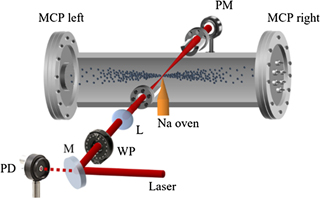
Figure 2. The experimental apparatus and associated optics. The experimental setup includes a steering mirror (M), half-wave plate (WP), lens (L), sodium oven, and a power meter (PM). The photodiode (PD) signal triggers the acquisition of electron arrival counts from the chevron microchannel plates (MCP).
Download figure:
Standard image High-resolution imageThe photoelectrons propagated along the chamber axis within a μ-metal shielded tube in a field-free region and were detected by the microchannel plate detectors (MCP, Del Mar Photonics MA34/2). A multiple-event time digitizer (FAST ComTech MCS6) with a 100 ps time resolution was employed for data acquisition by using start and stop channels. The start signal was obtained from a photodiode (PD) placed behind the mirror M (figure 2) and used for triggering the PCI counting card of the multiscaler. The stop signal produced by the detection event at the MCP detectors and amplified with a preamplifier (ZKL-2 Mini-Circuits) was recorded in a specific time bin corresponding to the arrival time relative to the start pulse. Angular distributions were measured by rotating the laser beam polarization with a half-wave plate controlled in an automated fashion and inserted into the path of the laser radiation. To set the laser intensity to desired values, a neutral density filter wheel was used. A power meter (PM), Ophir Nova II, was placed at the exit window of the ATI chamber to monitor the laser power during the experiment. All steps for controlling the experiment and recording data were automated by using a data acquisition card (National Instruments, DAQ PCI-MIO-16E-4) and LabVIEW 8.5 program.
3. Theoretical description
In the case of single-photon ionization, the PAD is described by the expression:

where dσ/dΩ is the differential cross section, σ is the integrated cross section, Ω is the solid angle, Pn (cos θ) is the Legendre polynomial of order n, β is the anisotropy or asymmetry parameter, which has values between (−1) and 2 [38, 39]. In the MPI case, the angular distributions of photoelectron can be described by the higher order Legendre polynomials. For n-photon ionization, angular distributions can be presented as [40]:

According to equation (2), the ionization of sodium to the continuum 0th order ATI requires Legendre polynomials up to 8th order, since for this 4 photons are needed. For a higher order ATI, higher order Legendre polynomials are required. Although this traditional approach formally describes angular dependences, in the next section we describe a different approach that better presents the ATI physics of sodium.
3.1. Contributions to ATI peaks with different orbital quantum numbers
Now we seek to obtain approximations for the probability of photoelectrons with different states after ionization. The atom can be described by electron orbitals representing the bound energy states. The atomic wave functions of the bound states represent standing (or stationary) waves of the atomic electrons, whereas the continuum energy states of the electrons are represented by wave functions describing propagating waves. The wave function of the continuum waves in momentum space can be expressed as a sum of scattered partial waves:

where  are the spherical harmonics for an orbital quantum number ℓ and magnetic quantum number m, while k is the magnitude of the momentum vector
  . The angles θ and ϕ represent the polar and azimuthal angles, respectively in the momentum space and are measured with respect to the laser polarization direction. The amplitudes Aℓ
(k) describe the radial distribution of the wave function.
. The angles θ and ϕ represent the polar and azimuthal angles, respectively in the momentum space and are measured with respect to the laser polarization direction. The amplitudes Aℓ
(k) describe the radial distribution of the wave function.
We can make several simplifying assumptions. First, note that spherical harmonics for m > 0 do not have a preferential orientation along the laser polarization. This means that there are all possible values of the azimuthal angle ϕ for these continuum waves. Since in the experiment we ionize an ensemble of sodium atoms, averaging over all possible ϕ should result in complete destructive interference at the detector. Consequently, we can assume m = 0.
Second, note that a three-photon transition from the 3s ground-state to either 5p or 4f results in the atom occupying an odd orbital, since ℓ = 1 for the p and ℓ = 3 for f orbitals. This means that a one photon transition from 5p (4f) to the 0th order continuum level results in a wave function composed of only even ℓ values (see figure 1). Similarly, a transition from the 0th order to the 1st order in the continuum yields a wave function of only odd ℓ values. So the wave function  in equation (3) can be separated into even series
  for the (0th, 2nd, ...) order photoelectron peaks and odd series
  for the (1st, 3rd, ...) orders:

and

where Pℓ (cos θ) are the Legendre polynomials for m = 0, and aℓ (k) are the complex-valued probability amplitudes defined by:

Here we have omitted the time dependence t in  and aℓ
(k) to simplify the notation. But note that the k dependence in aℓ
(k) also specifies the kinetic photoelectron energy Ek
= (ℏk)2/2me and the ATI peak order such that aℓ
(k) ∝ exp(−iEk
t/ℏ).
and aℓ
(k) to simplify the notation. But note that the k dependence in aℓ
(k) also specifies the kinetic photoelectron energy Ek
= (ℏk)2/2me and the ATI peak order such that aℓ
(k) ∝ exp(−iEk
t/ℏ).
Now, to find the relative contribution of the continuum waves to the photoelectron spectrum, we use a least-squares fit between the probability density  and our experimental data for each ATI spectral peak (k is assumed constant) as a function of θ. For the four- and six-photon ionizations of sodium the wave function of equation (4) was used to fit the probability density, while equation (5) was used for five- and seven-photon ionizations. The fit parameters aℓ
(k) are then normalized to find the contributions ρℓ
(k) to probability density of different continuum waves:
and our experimental data for each ATI spectral peak (k is assumed constant) as a function of θ. For the four- and six-photon ionizations of sodium the wave function of equation (4) was used to fit the probability density, while equation (5) was used for five- and seven-photon ionizations. The fit parameters aℓ
(k) are then normalized to find the contributions ρℓ
(k) to probability density of different continuum waves:

3.2. TDSE simulations
The TDSE calculations were performed with Qprop 3.2 [41], which incorporated the time-dependent surface flux (t-SURFF) method [42] in combination with the i-SURFV approach [43] for calculation of photoelectron spectra. This program calculates photoelectron spectra by solving TDSE

in a single active electron approximation with a Hamiltonian that includes the effect of the laser field in velocity gauge

where  is the vector potential in dipole approximation (with the electric field expressed as
  ),
),  is the binding potential of the atom, and
  is the imaginary potential introduced to absorb unwanted reflections from the numerical grid boundary. For our calculation we used the default Vim potential, and the binding potential had the Hellmann pseudopotential form [44]
This binding potential has the following properties. When the valence electron is close to the atomic core, r < α−1, the short-range potential mimics a repulsive potential. For larger distances from the core, 1/α < r < Rco, the potential approaches the Coulomb potential. With the t-SURFF method the photoelectron spectrum is calculated from the probability flux through a surface with the radius Rl located sufficiently far, where the binding potential practically vanishes. The i-SURFV approach reduces the calculation time by using a time-independent Hamiltonian after the decay of the laser field. In the calculations we accepted Rco = 10 a.u. and the t-SURFF boundary Rl = 200 a.u.. The laser field was approximated as

with the FWHM pulse duration τ = 58 fs and T = 2.67 fs.
The field amplitude in atomic units  a.u. was determined by the experimental intensities I = 2 × 10 13 W cm−2 and I = 1 × 10¹³ W cm−2. By performing imaginary time propagation, we determined the ionization potential (the energy of the 3s ground state E3s
) and the energies of the excited states. With the parameters of the binding potential A = 20, a = 2.5137, Rco = 30 a.u. the calculated values for Na are close to the experimental values [44] (see table 1). With the grid step sizes ∆t = 0.01 a.u. and ∆r = 0.04 a.u. typically calculation time of about 7 hours was required on a PC with a four-core, i7, 3.5 GHz processor.
a.u. was determined by the experimental intensities I = 2 × 10 13 W cm−2 and I = 1 × 10¹³ W cm−2. By performing imaginary time propagation, we determined the ionization potential (the energy of the 3s ground state E3s
) and the energies of the excited states. With the parameters of the binding potential A = 20, a = 2.5137, Rco = 30 a.u. the calculated values for Na are close to the experimental values [44] (see table 1). With the grid step sizes ∆t = 0.01 a.u. and ∆r = 0.04 a.u. typically calculation time of about 7 hours was required on a PC with a four-core, i7, 3.5 GHz processor.
Table 1. Comparison of calculated and experimental [44] values of energy levels for Na presented in a.u. and eV. The relative difference  in % is also shown.
| Na | −Ecalc a.u. (eV) | −Eexp a.u. (eV) | ΔE/E, % |
|---|---|---|---|
| 3s | 0.18881(5.136) | 0.18886(5.137) | −0.03 |
| 3p | 0.11235(3.057) | 0.11156(3.035) | 0.7 |
| 4s | 0.07024(1.962) | 0.07161(1.949) | −1.9 |
| 3d | 0.05540(1.508) | 0.05589(1.520) | −0.9 |
| 4p | 0.05130(1.395) | 0.05089(1.384) | 0.8 |
| 5p | 0.02937(0.799) | 0.02922(0.795) | 0.5 |
| 4f | 0.03123(0.850) | 0.03123(0.850) | 0.0 |
| 5f | 0.01996(0.543) | 0.01947(0.530) | 2.5 |
| 6p | 0.01881(0.511) | 0.01874(0.510) | 0.4 |
| 7p | 0.01050(0.286) | 0.01433(0.390) | −27 |
4. Experimental results
4.1. ATI energy spectrum
By measuring time-resolved photoelectron arrivals the ATI peaks can be obtained. The counter records the time it takes for an electron to travel from the ionization region to the MCP. Then time-of-flight (TOF) can be converted into an energy spectrum using the simple kinetic energy equation:

where me is the electron mass, t is the measured time; L = 0.40 m, the distance between ionization region and the MCP and the time delay δt = −3.9 ns are determined by the experimental setup. The TOF spectrum and the converted energy spectrum at the intensity of 2 × 10¹³ W cm−2 showing the ATI peaks from zero order to third order are depicted in figures 3(a) and (b). From the energy level diagram of figure 3 the well pronounced peaks in the spectrum can be identified as arising from the ionization pathway through the 5p(4f) level. The peak having an energy of ∼0.8 eV represents photoelectrons from 5p and 4f, while the peak at ∼2.35 eV shows the first order ATI peak of 5p(4f). As expected, ATI peaks are separated by one photon energy of 1.55 eV for 800 nm.

Figure 3. The upper panel shows the TOF spectrum of the photoelectrons, while the lower panel presents the ATI energy spectrum. The data in the upper panel was converted to kinetic energy and presented in a semi-log plot in the lower panel. The ionizations from the 5p(4f), 6p, and 7p states are observed.
Download figure:
Standard image High-resolution image4.2. Photoelectron angular distributions
Here, we discuss experimental measurements of PADs resulting from the ionization of atomic sodium. By changing the angle between the laser polarization and the direction of the electron flight the angular distribution of each of the ATI peaks was measured. Sodium atoms were ionized through the absorption of 4 or more photons. ATI 5p(4f) peaks up to third order were observed, and PADs of these peaks were measured. PADs in the MPI regime depend on the number of photons involved in the transitions, including those to intermediate levels. The 5p(4f) peaks are produced through the process 3s → → 4s → 5p.(3s → → → 4f), where each arrow indicates one photon, so the process for 5p the energy level involves 2 photons on the first step of ionization and one photon on the second step. The ionization from the 5p(4f)-level can go with the absorption of one or more photons giving rise to different ATI orders. In figures 4 and 5, PADs for the zero and higher ATI orders are shown for a laser polarization angle varied from 0° to 90° at the intensities of 2 × 10¹³ W cm−2 and 1 × 10¹³ W cm−2. It is clearly seen that electron yields depend on the laser polarization angle. In figure 6, polar plots present experimental PADs for the 5p(4f) ATI peaks, which were measured from 0° to 90° and reflected for 90° to 180° interval for better viewing. Solid lines show the least root-mean-square fits of the expressions of  with
with  described by equations (4) and (5) to the measured angular distributions.
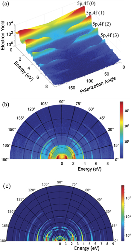
Figure 4. ATI spectra at the intensity of 2 × 10¹³ W cm−2 (a) experimental 3D plot measured from 0° to 90° and reflected to 90° to 180° for better viewing, (b) polar plot of the same data, (c) calculation with TDSE.
Download figure:
Standard image High-resolution image
Figure 5. ATI spectra at the intensity of 1 × 10¹³ W cm−2 (a) experimental 3D plot measured from 0° to 90° and reflected to 90° to 180° for better viewing, (b) polar plot of the same data, (c) calculation with TDSE.
Download figure:
Standard image High-resolution image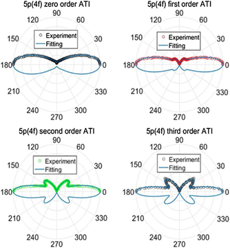
Figure 6. Photo-electron angular distributions of the sodium atom at the intensity of 2 × 10¹³ W cm−2. The upper panel shows angular distributions of zero and first order ATI, while the lower panel shows angular distribution of the second and third order ATI through the 5p(4f) state. Dotted upper portions of the plots show experimental data and lower portions with thin solid lines show fitting curves according to equations (4) and (5).
Download figure:
Standard image High-resolution imageFor the zero order ATI peak, requiring the minimal number of the absorbed photons, the angular distribution shows anisotropic behavior with a maximum at 0° (180°), a minimum at 90°, and a small side lobe at ∼60°. For the first, second, and third ATI peaks, the side lobes in the angular distributions are more pronounced. We also observed that with the increasing ATI order the position of the maximum electron yield in the side lobes is shifting. For example, for the 0th order ATI peak the maximum electron yield of the side lobe is at ∼60° while for the third order this maximum is observed at ∼40°.
Another observation is that the width of the angular distribution is becoming narrower with the increasing ATI order. PADs for above-threshold ionization of sodium atom are sharply peaked along the laser polarization direction. This can be expected since electron velocities tend to align in the direction of laser field force [45]. Having sharply peaked angular dependence at 0° and 180° can also be attributed to the superposition of all three s, d and g partial waves [46]. The reason PADs become more elongated along the laser polarization direction is due to the contribution of higher orders of partial waves with the increasing number of photons [21], which also leads to higher electron energies and more anisotropic behavior.
4.3. Dependence on intensity
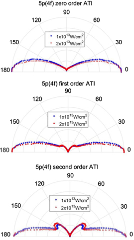
In figure 7 angular distribution of the zero, first and second order ATI from the 5p(4f) state at the intensities of 2 × 10¹³ W cm−2 and 1 × 10¹³ W cm−2 are compared. The third order ATI peak is not strong enough to be analyzed, so it is excluded.
Figure 7. Comparison of the angular distributions of the zero, first, and second order 5p(4f) ATI peaks at the intensities of 2 × 10¹³ W cm−2 (red) and 1 × 10¹³ W cm−2 (blue).
Download figure:
Standard image High-resolution image
As can be seen from figure 7, the twofold increase of the intensity did not qualitatively change the PADs. The number of side lobes is the same, but their shape somewhat varies for different intensities, which can be due to the dynamic Stark shift [16] and altered probabilities of different electron ionization pathways with changes of the laser intensity. Since zero order ATI requires four photons, the fitting using equation (2) with n = 8 was performed. Similarly, our data for the first order ATI peak are fitted well when the equation (2) includes terms up to n = 10 and for the second and third order ATI peaks, the equation (2) includes terms up to n = 12 and n = 14, respectively. Experimental fitting parameters for each ATI peak are shown in table 2.
Table 2. Fitting parameters σ and β of equation (2) for angular distributions of the ATI peaks of different orders at the intensities of I0 = 2 × 10¹³ W cm−2 and  .
.
| 5p(0) | 5p(1) | 5p(2) | 5p(3) | ||
|---|---|---|---|---|---|
| σ | I0 | 0.1588 | 0.1329 | 0.1792 | 0.1828 |
| I0/2 | 0.1775 | 0.1431 | 0.1789 | — | |
| β2 | I0 | 0.3638 | 0.3138 | 0.3325 | 0.3154 |
| I0/2 | 0.4173 | 0.3478 | 0.3515 | — | |
| β4 | I0 | 0.2663 | 0.1542 | 0.0160 | 0.0904 |
| I0/2 | 0.2715 | 0.1923 | 0.0397 | — | |
| β6 | I0 | 0.1831 | 0.1883 | 0.0779 | 0.0039 |
| I0/2 | 0.1278 | 0.2028 | 0.1511 | — | |
| β8 | I0 | 0.0894 | 0.1871 | 0.2139 | 0.1868 |
| I0/2 | 0.0935 | 0.1117 | 0.1911 | — | |
| β10 | I0 | — | −0.0794 | 0.1614 | 0.1783 |
| I0/2 | −0.0155 | 0.0549 | — | ||
| β12 | I0 | — | — | 0.0214 | 0.1508 |
| I0/2 | — | −0.006 | — | ||
| β14 | I0 | — | — | — | 0.0038 |
| I0/2 | — | — | — | — | |
| Fit error (%) | I0 | 0.79 | 1.07 | 1.54 | 2.58 |
| I0/2 | 0.46 | 0.41 | 0.78 | — |
Fitting the angular dependences with equation (2) gives their analytical description, however in the next section we discuss contributions of different ionization pathways and introduce fitting based on their contributions.
5. Discussion
For our data, the relative density values of the threshold (0th ATI) peak show significant ionization through both 5p level (the ionization channels with 2 + 1 + 1 and 3 + 1 photon) and 4f level (3 + 1 photon) REMPI (see table 3). For the threshold (0th order) peak, ionization from 5p (ℓ = 1) is restricted to the s (ℓ = 0) and d (ℓ = 2) continuum waves, while ionization from 4f (ℓ = 3) is restricted to contributions of the d (ℓ = 2) and g (ℓ = 4) waves (see figure 1).
Table 3. The relative probability density ( , equation (7)) and phase (Δ(k), equation (13)) in degrees for different ATI orders for laser intensities I0 = 2 × 10¹³ W cm−2 and
  .
.
| ATI orders | |||||||||
|---|---|---|---|---|---|---|---|---|---|
| 0th | 1st | 2nd | 3rd | ||||||
| Orbitals | Intensity | ρ | Δ | ρ | Δ | ρ | Δ | ρ | Δ |
| s | I0 | 0.23 | 278 | — | — | 0.19 | 233 | — | — |
| I0/2 | 0.20 | 191 | — | — | 0.10 | 252 | — | — | |
| p | I0 | — | — | 0.46 | 255 | — | — | 0.49 | 174 |
| I0/2 | — | — | 0.39 | 186 | — | — | — | — | |
| d | I0 | 0.47 | 231 | — | — | 0.22 | 201 | — | — |
| I0/2 | 0.70 | 241 | — | — | 0.38 | 315 | — | — | |
| f | I0 | — | — | 0.27 | 167 | — | — | 0.06 | 298 |
| I0/2 | — | — | 0.54 | 107 | — | — | — | — | |
| g | I0 | 0.30 | 202 | — | — | 0.29 | 99 | — | — |
| I0/2 | 0.10 | 272 | — | — | 0.50 | 28 | — | — | |
| h | I0 | — | — | 0.27 | 171 | — | — | 0.08 | 320 |
| I0/2 | — | — | 0.06 | 92 | — | — | — | — | |
| i | I0 | — | — | — | — | 0.30 | 137 | — | — |
| I0/2 | — | — | — | — | 0.02 | 24 | — | — | |
| j | I0 | — | — | — | — | — | — | 0.37 | 260 |
For the intensity 2 × 10¹³ W cm−2the 3 + 1 REMPI from the 3s through 4f accounts for 30% of the g-wave threshold electron yield. While the 2 + 1 + 1 and 3 + 1 REMPI through 5p make up 23% of the s-wave yield. Since ionized electrons from 5p and 4f constructively interfere in the d-wave 0th order peak, the individual contributions from each bound state cannot be separated. Nonetheless, their combined ionization into the d-wave is 47%. In higher order peaks, the 1st order h-wave, 2nd order i-wave and 3rd order j-wave have ℓ values that are too large for ionization from 5p. So these electrons must respectively arise from 3 + 2, 3 + 3 and 3 + 4 REMPI from the 3s ground state through the 4f Rydberg energy level.
At the lower laser intensity of (1 × 10¹³ W cm−2), our experimental measurement shows a general shift of the electron populations away from larger ℓ valued continuum waves as compared to the higher intensity (see table 3). For example, the 0th order peak has a comparable s-wave yield (20%) to the higher intensity experiment. However, for 1 × 10¹³ W cm−2 there is much more d-wave yield (70%) and much less g-wave (10%) than in the 2 × 10¹³ W cm−2 case. This suggests that (2 + 1 + 1) REMPI through 5p is the dominant ionization channel at the lower intensity. This observation can be explained by the differing photon orders needed to populate the 5p versus 4f. Because of the two-photon intermediate resonance between the ground state and 4s, the 5p state can be more efficiently populated at lower intensities than the three-photon 4f transition. Thus, the (3s–4s) Rabi oscillations act as a reservoir of electrons for REMPI through 5p [47–49]. But as intensity increases, three-photon processes (i.e. 3s–4f) increase in efficiency as they simultaneously Stark-shift into resonance. The trend toward higher intensities populating higher ℓ valued continuum waves was predicted theoretically [32], where simulations showed more REMPI through the 4f state at 8.8 × 10¹³ W cm−2 than at 3.5 × 10¹³ W cm−2.
The complex amplitudes aℓ (k) can be expressed in terms of their phase Δ:

In table 3, we show the phase Δ for each continuum wave and peak order for intensities 2 × 10¹³ W cm−2 and 1 × 10¹³ W cm−2 respectively. There are two potential contributions to phase for continuum waves. The first involves an ℓ-dependent scattering phase shift δℓ
of the outgoing waves, which arises from the scattering of partial waves with the Coulomb potential of the atom. A second source of phase shift involves the time-dependence of the wave function, where  . This implies that each ATI peak order is accompanied by a phase shift proportional to its energy. The comparison of experimental results with calculations based on TDSE presented in figures 4 and 5 shows that the positions of the ATI peaks, the strong decrease of the higher order ATI peaks and anisotropy of PADs with strongly pronounced maxima at from 0° and 180° are reproduced quite well. However, in some finer features, such as side angular lobes and fine structure of energy distribution for different ATI orders noticeable differences between experimental and theoretically calculated distributions are observed.
6. Conclusions
In this work, we have shown experimental results for MPI of sodium atoms in the near infrared spectral region. Kinetic energies of the photoelectrons were determined by converting the TOF spectrum to the kinetic energy spectrum. Ionization pathways through the intermediate 5p, 6p and 7p states were identified in the energy spectrum. Angular distributions of the photoelectrons ionized via the 5p state were investigated for the ATI peaks up to the third order. The analytical description of angular dependences was obtained by fitting the experimentally measured photo-electron angular distributions with Legendre polynomials. The insights into contributions of different ionization channels were obtained by presenting the electron wavefunctions as superpositions of s, p, ...j states with different orbital angular momenta that were presented as sums of Legendre polynomials with complex-valued probability amplitudes. This approach allowed evaluating the contributions to the probability density and phases of continuum waves with different orbital angular momenta based on experimental data. Angular distributions show anisotropic behavior with maxima at 0° and minima at 90°. There are also side lobes with maxima between 60° and 40° depending on the ATI order. The side lobes are more pronounced for the higher order ATI peaks. We observed that the maximum point of the side lobes is shifting to smaller angles with the increasing ATI order. The TDSE calculations of the ATI spectra in a single active electron approximation show agreement with the experiment of most prominent features, while in details of angular and energy distributions some differences are observed. Finally, we concluded that angular distributions of the photo-electrons do not depend significantly on the laser intensity, as we observed only slight variations in the angular distributions when the intensity was changed twofold.
Acknowledgments
This work was supported by the Robert A Welch Foundation Grant No. A1546. Y Boran acknowledges support from the Ministry of National Education of the Republic of Turkey. We thank V Tulsky for advice with TDSE calculations.
Data availability statement
The data generated and/or analysed during the current study are not publicly available for legal/ethical reasons but are available from the corresponding author on reasonable request.
Appendix.: Error analysis
The ATI spectra measured at each angle were acquired over a fixed time interval. Therefore, we assume that the dominant source of noise in the experiment comes from Poisson-noise which has a Poisson distribution. Gaussian (constant background) noise, instrumentation noise and outliers are assumed negligible. For any fixed measurement interval, the Poisson distribution has a standard deviation (SD) equal to the square root of the mean count rate.
The SD of the ionization data as a function of θ was approximated using two different methods. These methods were compared to ensure that our fit function could reasonably replicate the true probability density function. In the first method, we use the least-squares fit of the data  over the angle θ as the mean values of the probability density. Then we calculated the standard deviation SD1 between the data and the density. In the second method, we approximated the Poisson SD by taking the square root of the data directly where
  . In table 4 below, we list the percent deviation (PD) calculated with each method for all ATI peak orders, where the PD is defined by:

Table 4. The percent deviation for the density least-squares fit (PD1) and Poisson noise model (PD2).
| Error for ATI peak order | |||||
|---|---|---|---|---|---|
| 0th | 1st | 2nd | 3rd | ||
| 1 × 10¹³ W cm−2 | PD1 | 1.05 | 5.4 | 9.5 | n/a |
| PD2 | 1.06 | 3.3 | 9.9 | n/a | |
| 2 × 10¹³ W cm−2 | PD1 | 0.86 | 4.16 | 6.42 | 20.19 |
| PD2 | 0.83 | 2.38 | 6.14 | 15.45 | |
At both intensities, the PD increases with increasing ATI order from the threshold peak to the 3rd order peak due to a decrease in the count rate at higher electron energies. The PD between the data and the fit is within 2% for the 0th, 1st and 2nd order ATI peaks. For 1 × 10¹³ W cm−2, the electron count rate for the 3rd order peak was too low to make a meaningful estimate of the SD.