

Abstract
Ionic polymer metal composites (IPMCs) are an emerging class of soft active materials that are finding growing application as underwater propulsors for miniature biomimetic swimmers. Understanding the hydrodynamics generated by an IPMC vibrating under water is central to the design of such biomimetic swimmers. In this paper, we propose the use of time-resolved particle image velocimetry to detail the fluid kinematics and kinetics in the vicinity of an IPMC vibrating along its fundamental structural mode. The reconstructed pressure field is ultimately used to estimate the thrust produced by the IPMC. The vibration frequency is systematically varied to elucidate the role of the Reynolds number on the flow physics and the thrust production. Experimental results indicate the formation and shedding of vortical structures from the IPMC tip during its vibration. Vorticity shedding is sustained by the pressure gradients along each side of the IPMC, which are most severe in the vicinity of the tip. The mean thrust is found to robustly increase with the Reynolds number, closely following a power law that has been derived from direct three-dimensional numerical simulations. A reduced order distributed model is proposed to describe IPMC underwater vibration and estimate thrust production, offering insight into the physics of underwater propulsion and aiding in the design of IPMC-based propulsors.
Export citation and abstract BibTeX RIS
1. Introduction
Ionic polymer metal composites (IPMCs) are a novel class of smart materials that are finding increasing application as actuators, sensors, and energy harvesters in underwater environments [1, 2]. IPMCs generally consist of a hydrated ionomeric membrane plated by noble metal electrodes and neutralized by mobile counterions [1, 2]. Sensing and energy harvesting in IPMCs are often associated with variations in the electrochemical potential in response to changes in the charge concentration induced by mechanical deformations of the backbone ionomer [3–7]. Conversely, IPMC actuation can be related to Maxwell stress and osmotic pressure caused by the electric field and charge redistribution from an imposed voltage difference across the electrodes [7–10].
A key application of IPMCs is within biomimetic miniature swimmers, as originally proposed in [11] and later developed in the technical literature [12–23]. In these studies, vibrating IPMCs are utilized as underwater propulsors, based on their ability to operate in wet environments with low actuation voltage, fast actuation response, high flexibility, and light weight [18, 24]. In [12], an IPMC-based tadpole robot was designed and realized, and the thrust and swimming speed were measured as functions of the vibration frequency. In [14], the thrust generated by IPMCs with patterned electrodes was investigated using a fixed propulsor connected to a load cell. Jellyfish robots incorporating IPMCs have been studied in [15, 19]. In [15], a curved IPMC actuator was considered and the thrust and swimming speed of the jellyfish robot were measured. In [19], flat IPMCs were instead attached to bell-shaped polymer films, and the swimming speed of the robot was experimentally measured. In [13, 17, 20–22], IPMCs were used as the tail of robotic fish of varying dimensions, and theoretical insights were proposed to shed light on the physics of propulsion. In [16], a robotic ray was designed and realized using two IPMC wings. In [23], the possibility of exploring patterned IPMCs to enable bending and twisting motions for underwater propulsion of robotic fish was demonstrated. A comparison between IPMC-based biomimetic swimmers and other robots has been recently presented in [25], focusing on scaling laws adapted from animal swimming [26].
As the interest in IPMC-based underwater propulsion grows [18], the need of understanding and predicting the hydrodynamics generated by an IPMC vibrating under water in a viscous fluid has become more pressing [17, 20–22, 27–30]. In [27], a two-dimensional (2D) numerical study on the flow induced by an IPMC vibrating along its fundamental mode was presented. Numerical results presented therein demonstrate the central role of vorticity generation and shedding from the IPMC tip on thrust generation. The effect of higher modes in IPMC-based underwater propulsion was investigated in [12–14, 31–33]. In [30], 3D direct numerical simulations were conducted to understand the role of the aspect ratio, width-to-length ratio, on the flow physics induced by the IPMC. Beyond confirming the important role of coherent fluid structures in the vicinity of the IPMC tip, 3D simulations highlight a number of salient flow features which are not captured by 2D models.
In synergy with design-oriented experimental studies [17, 20–22], the hydrodynamics generated by IPMCs vibrating in quiescent fluids has been studied in [28, 29] using particle image velocimetry (PIV). In [28], time-average PIV was used to estimate the thrust production and isolate the formation and orientation of fluid jets in the vicinity of the IPMC tip. In [29], time-resolved PIV was utilized to refine the thrust estimation and explore a wider range of IPMC geometries.
Here, we seek to bridge numerical simulations and experimental studies through a refined PIV-based investigation of the fluid kinematics and kinetics generated by a vibrating IPMC. PIV results are utilized to examine the vorticity field and improve our understanding on flow physics generated by a vibrating IPMC. By using a pressure reconstruction technique on PIV data [34], we estimate the pressure field in the fluid along with the produced thrust. While pressure techniques have been implemented across a number of fluid dynamics problems [34], their use in the study of fluid-structure interaction problems is relatively limited [35–38]. An even more elusive question entails the study of fluid-structure interaction associated with the vibrations of smart materials in otherwise quiescent fluids.
Experiments are conducted on an in-house fabricated IPMC cantilever excited by a sinusoidal voltage of varying frequency applied across its electrodes. The IPMC vibration is measured from raw images to calculate salient non-dimensional flow parameters and aid in the pressure reconstruction from PIV data, which requires knowledge of the IPMC location. Experimental results are compared to numerical solutions [27, 30] and other experimental studies, including observations on piezoelectrics and servomotor-controlled passive foils [28, 29, 39–41]. To aid in the interpretation of the experimental results and offer insight into the possibility of designing IPMC propulsors, a distributed model for IPMC underwater vibration and thrust production is presented. The modeling scheme is based on the framework presented in [7] for predicting IPMC actuation from fundamental physical and geometric parameters, Morison formula [42, 43] for estimating fluid-structure interaction, and the regression model in [30] for thrust estimation from non-dimensional flow parameters.
The paper is organized as follows. In section 2, we describe the experimental scheme and methods used for the study. In section 3, we present our experimental results, including IPMC vibration and the resulting fluid kinematics and kinetics. Conclusions are summarized in section 4.
2. Experimental scheme
The IPMC is fabricated in-house from commercial Nafion membrane foils N117, produced by DuPont de Nemours, through electroless chemical reduction of platinum salt [44, 45].  cations are selected as the mobile counterions species for fast actuator response [46]. The sample has a width
  , length
  , and nominal thickness
  , see figure 1. The mass per unit length of the sample is estimated from direct weight measurement to be
  . The bending stiffness and loss factor are
  and
and  , obtained from a free vibration experiment in air [47]. To determine the electrical properties of the IPMC, we measure the electric impedance using the 'AC impedance' technique on a CH Instruments 760D potentiostat [48].
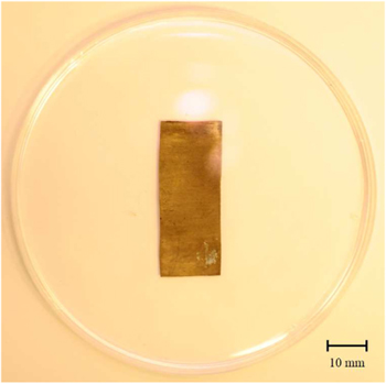
Figure 1. Picture of the IPMC in a Petri dish.
Download figure:
Standard image High-resolution imageFigure 2 displays the experimental setup for the underwater thrust analysis. To actuate the IPMC, we apply a voltage difference across the electrodes using two external  long copper sheets placed on one end of the sample. Thus, the free actuation length of the IPMC is
  . An ac voltage
  with amplitude
  and varying radian frequency ω is used to actuate the IPMC. The signal is generated with a Kenwood KAC-6202 power amplifier, which is connected to a Agilent 33210A function generator. We control the applied voltage by adjusting the output signal of the function generator. The sine-wave signal has a driving frequency
  ranging from 1 to
  with an increment of
  . The range of frequencies is selected to span the resonance band of the fundamental vibration mode of the IPMC in water on the basis of a preliminary theoretical analysis and pilot experiments. To control the magnitude of the applied voltage, we measure the voltage through a National Instruments data acquisition 9229 board via a custom Labview (www.ni.com/labview) code at a sampling rate of
  . Experiments are conducted in a transparent tank with dimension of 400 × 200 ×
  , filled with tap water at room temperature (the mass density per unit volume and the dynamic viscosity are taken as their nominal values of
  and
and  , respectively). The IPMC is stored in deionized water when not in use for the experiments.

Figure 2. Picture of experimental setup with overlaid nomenclature. In the inset, we display the IPMC used for the experiments.
Download figure:
Standard image High-resolution imageTo extract the IPMC deflection and flow velocity field around the IPMC during actuation, a Phantom high speed camera with DynamicStudio software (www.dantecdynamics.com) records both the IPMC vibration and the flow field for 3 s. The resolution of the recorded images is 1632 × 1200 pixels (131 ×  ), and the acquisition rate is set so that it is 100 times the driving frequency,
  . A RayPower laser source illuminates the mid-plane of vibration and silver-coated hollow glass spheres with diameter of
  are used as particle seeding for PIV analysis. Standard PIV is inherently 2D, and as such the PIV-based experimental analysis does not capture or elucidate 3D phenomena. To track the tip deflection of the IPMC, the same images are analyzed using a dedicated tracking software Xcitex ProAnalyst (www.xcitex.com).
To enhance the resolution of the flow velocity, we adjust the number of images skipped in the image sequence following [29]. Such a time delay allows sufficient particle motion when cross-correlating images during PIV analysis; specifically, the first image is cross-correlated with the sixth, the second with the seventh, and so on. The PIV images are analyzed using an open-source Matlab (www.mathworks.com) code 'PIVlab' [49], which is based on a Fast Fourier transform cross-correlation algorithm and a decreasing interrogation area size of 64 × 64, 32 × 32, 16 × 16, and 8 × 8 pixels [50–52]. A 2 × 3 Gaussian interpolation is used for subpixel interrogation [53]. The fluid region occupied by the IPMC is masked in the images by a rotating rigid block of thickness  and length equal to the IPMC. The block rotates about the base and its tip displacement corresponds to the measured IPMC tip displacement. Note that the larger thickness of the block is necessary to fully mask the IPMC and any associated laser reflections from the surface during the IPMC motion. A schematic of the experimental configuration is presented in figure 3.
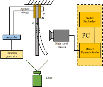
Figure 3. Schematic of the experimental setup.
Download figure:
Standard image High-resolution image3. Results
3.1. IPMC vibration
Figure 4 shows the time trace of the tip displacement of the IPMC at the driving frequency  . Raw motion data are fitted with a sine-wave by utilizing the Matlab built-in function 'fit,' to demonstrate that the tip displacement is well described by a harmonic signal at the input frequency. In figure 5(a), we display the peak tip displacement
  as a function of the input frequency. The peak tip displacement decreases as the input frequency increases, likely due to the hydrodynamic damping from the encompassing fluid [54]. The hydrodynamic damping tends to mask the underwater resonance of the IPMC, which can be seen from the peak tip velocity in figure 5(b). Therein, we note that the fundamental resonance frequency is located around approximately
  .
.

Figure 4. Tip displacement of the IPMC at  . The black solid line is the tracking data, and the red dashed line is the fitted line.
  is the period of oscillation.
Download figure:
Standard image High-resolution image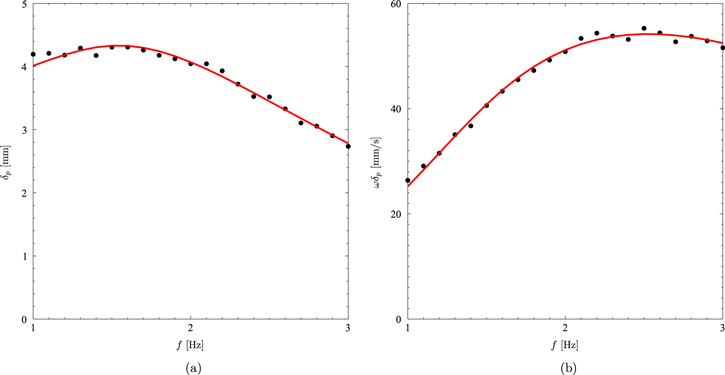
Figure 5. (a) Peak tip displacement as a function of the input frequency. (b) Peak tip speed as a function of the input frequency. Black markers are the experimental data, and red solid lines are model predictions with experimentally identified parameters.
Download figure:
Standard image High-resolution imageTo interpret the experimental findings, we model the IPMC vibration by combining our recent physics-based modeling framework for IPMC actuation [7] with the classical Morison formula [42, 43] that describes fluid-structure interactions for slender bodies. Within this framework, the IPMC vibration is governed by the following equation:

where  is the deflection (
 ),
),  is the hydrodynamic forcing from the encompassing fluid, and
  is the structural damping [55].
The boundary conditions are as follows [42, 56]:


where M(t) is the bending moment generated by counterion migration within the IPMC. Such a bending moment is associated with ion mixing and electric polarization within the ionomer core and the electrodes [7]. We hypothesize that the time scale of the IPMC deformation is considerably slower than the chemoelectric response so that the bending moment M(t) can be described from the quasi-static solution presented in [7], which posits a simple functional dependence of M(t) on the square of the applied voltage, without a significant dependence on the mechanical deformation. As a result, we simply treat the bending moment as a known function of time of the form  .
.
Following [42, 43], we write the hydrodynamic loading  as
as

where  is the added mass coefficient and
  is the hydrodynamic damping coefficient.
We approximate the structural damping with a simple hysteretic model, wherein the bending stiffness K is replaced in the frequency domain with the complex bending stiffness  , where
  is the imaginary unit [55].
Following [42], we utilize the Galerkin method to solve equation (1) with boundary conditions in equations (2a)–(2d). We use the first fundamental mode shape of a cantilever beam as a basis function, and we identify  ,
,  , and Mp by fitting the experimental data in figure 5(a) using the Mathematica built-in function 'Findfit' (www.wolfram.com). Following this procedure, we find
  ,
,  , and
, and  with a coefficient of determination
  . To illustrate the accuracy of the model, in figure 5, we report model predictions against experimental findings.
The experimentally identified hydrodynamic coefficient is slightly lower than typical experimental observations, whereby data on  are generally found to cluster in the vicinity of one and data on
  are often found in the range 10–20 [41–43, 54, 57]. Such discrepancies may be ascribed to the low aspect ratio
  of the IPMC, which favors 3D fluid-structure interactions [42, 43]. This hypothesis rests upon experimental observations in [42, 43], which indicate that both the hydrodynamic coefficients strongly decrease as the aspect ratio decreases, and computational results in [30], suggesting that the added mass effect is highly mitigated by 3D phenomena. Beyond the dependence on the aspect ratio, the hydrodynamic coefficients vary as functions of both the Reynolds (
 ), constructed by using the IPMC free length as the characteristic length in the flow, and the Keulegan–Carpenter (
 ) numbers, which quantify the role of viscous and convective phenomena in the flow field [41, 57–59].
The identified value of Mp is in line with results in [7]. Specifically, the value of Mp for an applied voltage of  can be retrieved using the same physical and geometric parameters in [7], namely, Faraday constant
  , gas constant
  , temperature
  , mobile counterion concentration
  , volume fraction of the ionomer in the composite layers
  , packing limit factor
  , permittivity ratio factor
  , and ionomer's semithickness
  , see [7] for detailed description. Only interfacial properties, such as ionomer's permittivity
  and composite layer's thickness
  are slightly modified with respect to [7] to reflect experimental observations, which are known to be highly influenced by specific fabrication conditions [48]. Specifically, the ionomer's permittivity is obtained from the measured impedance [48] and the composite layer's thickness is tuned to match the desired value of Mp.
3.2. Velocity field
In figures 6 and 7, we illustrate the instantaneous flow velocity and vorticity fields over one cycle of oscillation at  for 8 consecutive time instants from t = 0 until
  with step size of
  , where
  is the oscillation period. In figure 6, the contour variable is the velocity magnitude
  , normalized by the peak tip speed
  , where
  and
and  are velocity component along the x and y-axes, respectively. Note that when t = 0 and
  , the IPMC is not exactly parallel to the x-axis, due to a mild asymmetry of the IPMC motion caused by a slight initial waviness. In figure 7, the contour value is the normalized vorticity magnitude
  , where positive values refer to clockwise vorticity, and negative values indicate counterclockwise vorticity.
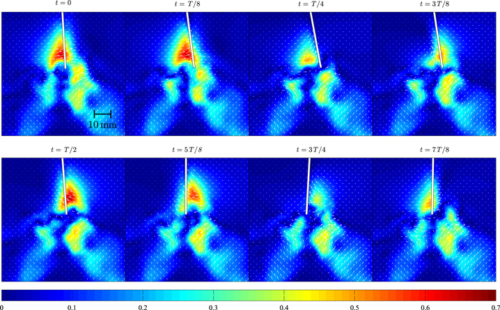
Figure 6. Contours of the non-dimensional velocity magnitude  for
for  (Re = 1416). The white block indicates the approximate IPMC position. The fluid flow is shown by the velocity vectors superimposed on the contours.
Download figure:
Standard image High-resolution image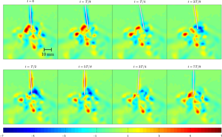
Figure 7. Contours of the non-dimensional vorticity magnitude  for
for  (Re = 1416). The white block indicates the approximate IPMC position.
Download figure:
Standard image High-resolution imageThe influence of the IPMC motion on the fluid flow is largely confined to its proximity, especially towards the tip of the IPMC, where we observe the shedding of vortices of alternating sign. In agreement with [28, 29], this results into the formation of two flow jets, as shown in figure 8(a), where we plot the mean flow field over an entire cycle computed from the full 0.66 s of recorded data (100 individual velocity fields), corresponding to 1 complete oscillation for  . In figure 8, we also present the mean velocity field for
  (figure 8(b)) and
  (figure 8(c)). In agreement with [28, 29], as the input frequency increases, the topology of the fluid jets changes, yet a clear dependency of the strength and angle with respect to Re is difficult to isolate. The interplay between viscous and inertial phenomena in the flow field has a central role in shaping the strength and configuration of the fluid jets originating at the IPMC tip.

Figure 8. Contours of the mean flow fields normalized by  at different frequencies. (a)
  , (b)
, (b)  , and (c)
  . The fluid flow is shown by the velocity vectors superimposed on the contours.
Download figure:
Standard image High-resolution image3.3. Pressure field
A pressure reconstruction method [36] is utilized to estimate the pressure distribution in the fluid surrounding the IPMC from the planar PIV data. Following [36], we neglect viscosity, gravity, and compressibility so that the pressure field is governed by the Poisson equation

where  is a kinematic source term written as

Dirichlet boundary conditions are imposed along the periphery of the PIV domain, whereby we assume that the pressure vanishes away from the IPMC. In addition, neglecting the local curvature of the vibrating IPMC, a homogeneous Neumann boundary condition  is imposed on the grid points close to the IPMC. The pressure field is computed using a custom Matlab script, similar to [36].
Figure 9 displays the non-dimensional pressure fields  for one oscillation cycle at the same intervals and frequency with figure 6. As the IPMC vibrates, the positive pressure mostly leads the motion of the IPMC while the negative pressure follows the IPMC [53], see
  and
and  in figure 6. As a result, the pressure difference of the fluid from the leading and trailing regions creates an opposing force to the IPMC motion [53], which is manifested through the added mass and hydrodynamic damping in equation (3). We note that the production of vorticity on the surface of the IPMC is directly proportional to the pressure gradient along the surface; thus, the concentrated regions of low and high pressure near the tip of the IPMC in figure 9 (see for example
  ) correspond to the phases at which vorticity is predominantly produced and subsequently shed in figure 8 [60].

Figure 9. Contours of the non-dimensional pressure magnitude  . The white block indicates the approximate IPMC position.
Download figure:
Standard image High-resolution imageFigure 10(a) presents the non-dimensional pressure difference across the IPMC along its length at the same intervals shown in figure 6. Specifically, the difference is calculated by subtracting the pressure on the right side from the left side of the white block in figure 9. The decrease in pressure magnitude in the vicinity of the tip of the IPMC can be ascribed to vortex shedding [30]. In agreement with [27, 30], the pressure difference is maximized in the vicinity of the IPMC tip. In figures 10(b) and (c), we display the non-dimensional pressure difference across the IPMC for  and
and  , similar to figure 8. Numerical results in [27, 30] suggest that the specific location where the maximum is attained should be influenced by the Reynolds number. However, the rather narrow range of Reynolds numbers, from 1018 to 1844, considered in this study does not allow for resolving variations in the pressure profile as a function of Re.
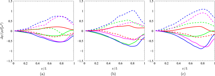
Figure 10. Non-dimensional pressure differences  across the IPMC for consecutive time instants. (a)
  , (b)
, (b)  , and (c)
  . Red solid, green solid, blue solid, purple solid, red dashed, green dashed, blue dashed, and purple dashed lines indicate t = 0,
  ,
,  ,
,  ,
,  ,
,  ,
,  , and
, and  , respectively.
Download figure:
Standard image High-resolution image3.4. Thrust produced by the vibrating IPMC
The thrust generated by the vibrating IPMC is computed using two methods: (i) integrating the reconstructed pressure on the IPMC, and (ii) performing a control volume analysis around the IPMC following [29].
Specifically, we compute the time trace of the thrust per unit width  by integrating the pressure obtained in section 3.3 on the outer surface of the rotating block that masks the IPMC through the Matlab built-in function 'trapz,' see figure 11. Following [27, 41], the thrust is fitted as the summation of a constant and a harmonic function with radian frequency twice the input frequency ω using the Matlab built-in function 'fit'. This behavior should be attributed to vorticity shedding at the IPMC tip, which is manifested through the generation and shedding of two coherent fluid structures per cycle [27]. Similar to numerical findings in [27], the thrust is minimized when the IPMC is in its neutral (flat) configuration and is maximized when the tip displacement is maximum [21, 23, 41].
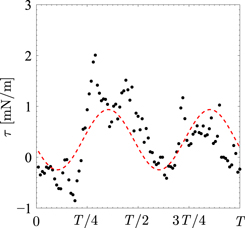
Figure 11. Computation of the thrust from the pressure field data. Black dots are experimental data and the red dashed line is the result of the fitting.
Download figure:
Standard image High-resolution imageAlternatively, the thrust of the IPMC is computed by performing a control volume analysis in a 2D region surrounding the IPMC following [29]. In our computation, we neglect momentum flux in the out-of-plane direction and utilize only planar PIV data; the expected uncertainty of such a computation should be within 10–20% as suggested in [29]. Neglecting gravity, viscosity, and compressibility, we find

where  is the boundary of the control surface, dl is a line element of
  , and nx and ny are the components of the unit outward of the control surface in the x and y directions. The control surface is approximately
  . The first two terms on the right hand side of equation (6) can be estimated directly from PIV data. In the evaluation of the last integral in the right hand side of equation (6), we use the pressure obtained in section 3.3 along the boundaries of the control surface. To compute the mean thrust per unit width
  generated by the actuating IPMC, equation (6) is integrated over a period. The average of the first term on the right hand side of equation (6) is assumed to be zero by assuming that the flow field is periodic.
Following [30], we calculate the non-dimensional thrust coefficient from the mean thrust, that is,

Figure 12(a) presents the non-dimensional thrust coefficient with the regression model presented in [30], based on 3D direct numerical simulations. Along with predictions from [30], in figure 12(a), we also display the thrust coefficient calculated from [27] on the basis of direct 2D numerical simulations. This comparison confirms the important role of 3D phenomena and the accuracy of the regression model in [30], which can aid in the design of underwater propulsors and specifically inform the selection of the aspect ratio that is often neglected in established modeling schemes [61, 62]. We comment that significant 3D phenomena are predominantly restricted to the vicinity of IPMC tip and are more relevant for lower aspect ratios [30].
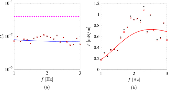
Figure 12. (a) Non-dimensional thrust coefficient. Black dots represent results from the control volume analysis and red crosses represent the direct integration of the pressure field. Blue solid and purple dashed lines represent the non-dimensional thrust coefficient proposed in [30] ( ) and from [27] (
 ), respectively. (b) Mean thrust per unit width. Black dots represent results from the control volume analysis and red crosses represent the direct integration of the pressure field. Red solid line represents theoretical predictions by combining the model in equation (1) with the regression model for the thrust coefficient proposed in [30].
Download figure:
Standard image High-resolution imageTo demonstrate the possibility of predicting IPMC thrust, we combine the distributed model in equation (1) with the regression model for the thrust coefficient illustrated in figure 12(a). Specifically, we utilize theoretical predictions in figure 5(b) to calculate the Reynolds number and use the regression model for  along with equation (7) to estimate the mean thrust per unit width. Theoretical results are presented in figure 12(b), superimposed to experimental data. The model is successful in predicting the trend of variation of the mean thrust and anticipating the presence of a maximum at approximately
  ; the model does tend to under-predict the mean thrust for vibration frequencies in the vicinity of
  , though the discrepancy is modest.
To compare our findings with the technical literature on thrust production of vibrating strips, in figure 13, we plot our data together with existing experimental results [21, 28, 29, 39–41]. Such data encompass IPMCs [21, 28, 29], piezoelectrics [39, 40], and servomotor-controlled passive foils [41]. The IPMC data in [21, 28, 29] share the same range of Reynolds numbers as our dataset, and consistently display similar thrust levels. The data in [21] are slightly larger than the rest; this discrepancy may be ascribed to the presence of a passive fin at the IPMC tip in [21]. Data in [39–41] show much larger thrust levels, which are in fact associated with higher Reynolds numbers. Experimental data presented therein refer to larger structures, whose characteristic length is approximately  [41],
[41],  [40], and
  [39] as compared to
  used in IPMCs. Servomotors and piezoelectrics afford higher tip speed compared to IPMCs, whereby data in [40, 41] encompass tip speeds as large as 0.62 and
  . In [39], the higher range of Reynolds number is associated with a considerably larger tip speed of
  , which compensates for the fact that the experiments are conducted in air.

Figure 13. Comparison of calculated thrust from both control volume analysis and pressure field with the experimental data from Aureli et al [21], Cen and Erturk [40], Eastman et al [39], Kopman and Porfiri [41], Peterson et al [28], and Prince et al [29].
Download figure:
Standard image High-resolution image
4. Conclusion
In this paper, we analyzed the hydrodynamics and thrust production of a centimeter-size IPMC vibrating under water. The input frequency was systematically varied from 1 to  to investigate the effect of Reynolds number on the fluid kinematics and kinetics. The Reynolds number was estimated by processing raw images to measure the IPMC tip vibration. Planar PIV was used to measure the flow velocity in the vicinity of the IPMC and a pressure reconstruction technique was utilized to estimate the pressure field and the thrust production. Two different approaches were proposed to estimate the thrust, that is, directly integrating the pressure field on the IPMC or performing a control volume analysis.
Our results indicate that IPMC vibration is accompanied by the robust generation and shedding of coherent fluid structures from the tip. Vortex advection, in turn, causes the formation of two fluid jets from the IPMC tip, whose topology is modulated by the Reynolds number in agreement with [28, 29]. Variations of the pressure field in the fluid are also localized in the vicinity of the IPMC, whereby the fluid tends to oppose IPMC motion during the whole vibration cycle. The pressure difference across the IPMC is maximized in the vicinity of the tip, where vorticity is formed in agreement with numerical predictions [27, 30]. Pressure variations are ultimately responsible for the production of a net thrust along the IPMC axis. The mean thrust per unit IPMC width increases with the Reynolds number attaining values as large as  , similar to [28, 29]. By comparing experimental predictions with numerical findings [27, 30], we confirm the role of 3D effects which substantially reduce the thrust production.
To aid in the analysis of experimental results and support the design of IPMC propulsors, we proposed a reduced order modeling scheme for IPMC underwater vibration and thrust production. The model is based on linear Euler–Bernoulli beam theory. IPMC actuation is treated using the framework presented in [7], and fluid-structure interaction is described using the Morison formula [42, 43]. Experimental data were used to calibrate the IPMC actuation model and identify the added mass and hydrodynamic damping coefficients of the Morison formula. The model allows for predicting IPMC underwater vibration from the input voltage across the whole range of excitation frequencies. The knowledge of the IPMC vibration is ultimately used in the regression model proposed by [30] to estimate the mean thrust produced by the IPMC. The overall framework, integrating PIV and IPMC modeling, is expected to assist in the design of biomimetic swimmers and improve our understanding of IPMC propulsors.
Acknowledgments
This work is supported by the National Science Foundation under grant numbers CMMI-0745753 and CBET-1332204, and the Mitsui USA Foundation. The authors also acknowledge the support of the Office of Naval Research through grant number N00014-10-1-0988 that allowed the acquisition of equipment used in this study. Finally, the authors wish to thank Mr Mohammad Jalalisendi and Mr Hubert Kim for their valuable help with PIV analysis and IPMC sample fabrication.