

Abstract
This paper presents a modified analytical model to study the sensing performance of a flexible capacitive tactile sensor array, which utilizes solid polydimethylsiloxane (PDMS) film as the dielectric layer. To predict the deformation of the sensing unit and capacitance changes, each sensing unit is simplified into a three-layer plate structure and divided into central, edge and corner regions. The plate structure and the three regions are studied by the general and modified models, respectively. For experimental validation, the capacitive tactile sensor array with 8 × 8 (= 64) sensing units is fabricated. Experiments are conducted by measuring the capacitance changes versus applied external forces and compared with the general and modified models' predictions. For the developed tactile sensor array, the sensitivity predicted by the modified analytical model is 1.25%/N, only 0.8% discrepancy from the experimental measurement. Results demonstrate that the modified analytical model can accurately predict the sensing performance of the sensor array and could be utilized for model-based optimal capacitive tactile sensor array design.
Export citation and abstract BibTeX RIS
1. Introduction
With the rapid growth of human–robot interaction and object manipulation, tactile sensors are indispensable for obtaining information about contact forces [1]. Capacitive tactile sensors, which feature high sensitivity and spatial resolution [2], have been widely utilized for robotic grasping [3], prosthesis hand motion [4] and biomedical surgery [5]. In these applications, tactile sensors are usually mounted onto curved surfaces. Thus, flexibility is required for the development of the tactile sensors. To realize flexibility, flexible electrodes and substrates have been utilized in the design of the tactile sensors [6].
For flexible capacitive tactile sensors, external force applied on the sensing unit will reduce the distance between the two capacitor electrodes, which will lead to the change of capacitance [7]. To improve the sensing performance of the capacitive tactile sensor, several methods have been presented. These methods can be classified into two types, including designing different types of capacitor electrodes and dielectric layers. For the capacitor electrodes, rectangular [8], triangular [9], comb-like [10, 11] and floating [12] electrodes have been utilized. By patterning the shape of the electrodes, the sensor can measure three-axial force and the spatial resolution can be improved. For the dielectric layer, air gap [13, 14], solid thin nano-needles film [15] and incompressible fluid sandwiched between two capacitor electrodes [16] have been utilized. The sensors using solid and fluid dielectric layer are less sensitive than those using air gap, but have a larger force measuring range. Compared to the air gap utilized as the dielectric layer, flexible solid PDMS features higher Young's modulus and could be used for large contact force measurement. Thus, solid PDMS film is selected and used as the dielectric layer for the developed capacitive tactile sensors array.
To study the sensing performance of the capacitive tactile sensor array, finite element modeling (FEM) has been widely utilized due to its high accuracy and the capability of modeling complex structures [4, 13, 17, 18]. For capacitive tactile sensor array, it usually has a multi-layer structure and each layer has a small thickness and large traverse area. For FEM modeling, it requires a large amount of meshes or mesh refinement to achieve mesh convergence [19], which limits the application of FEM in analyzing tactile sensor array. To solve this problem, analytical modeling, which features fast converge speed [20, 21], has been selected to study the sensing performance of the tactile sensor array and has become one goal of this research. Moreover, model-based structural optimization of the tactile sensor array could be achieved based on the developed analytical model. For analytical modeling of capacitive tactile sensors, Maier–Schneider et al [22] and Wang et al [23] have presented thin plate models to describe the deformation of the square membrane, which can be utilized to calculate the capacitance change of the tactile sensor with square electrodes. For the capacitive tactile sensor with circular electrodes, Meng et al [24] has established a 2D model to study the deformation in arbitrary plane crossing the center of the electrodes and obtained the relation between the pressure and capacitance. To predict the deformation of the capacitive electrodes, we previously developed a 3D analytical model [25], which assumes the Polyethylene Terephthalate (PET) substrate of the sensor is rigid to generate a two-layer plate structure and utilizes a linear function to describe the nonlinear relation between the deformation and coordinates of different layers of the sensing unit. These assumptions have led to 28% and 33% errors when predicting the deformations of edges and corners of the loading area, respectively. To accurately predict the deformation of the sensing unit, PET substrate should not be treated as rigid and the linear function should be replaced by a nonlinear one to describe the deformation tendency along layers of the sensing unit. Thus, a more accurate 3D analytical model needs to be established.
In this study, we develop a modified 3D analytical model to predict the deformation of the sensing unit and study the sensing performance of the flexible capacitive tactile sensor array. Firstly, the structural design of the capacitive tactile sensor array and its working principle are introduced. Based on the Ritz method, a modified analytical model is developed by dividing the sensing unit into the central, edge and corner regions. This is followed by tactile sensor array fabrication and experimental tests. Finally, results and discussions are conducted.
2. Design of the flexible capacitive tactile sensor array
Figure 1(a) shows the overview of the designed capacitive tactile sensor array, which consists of 8 × 8 sensing units. The overall dimensions of this sensor array are 35 × 35 mm. Spatial resolution, which is defined as the distance between the center points of two adjacent sensing units, is 4 mm. For each sensing unit, the upper and lower electrodes have the same thickness of 200 nm, which are generated on the upper and lower PET films, respectively, forming a capacitor. As shown in figure 1(b), the PET films have the same thickness with the value of 25 μm and a 20 μm-thick solid PDMS film serves as the dielectric layer which is sandwiched between the two PET films and electrodes. To concentrate the external force on the sensing unit, a PDMS bump with dimensions of 3000 × 3000 × 1000 μm is laminated on the upper PET film.
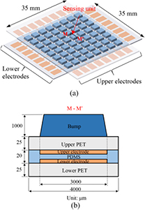
Figure 1. (a) Schematic view of the flexible tactile sensor array and (b) M–M' cross section of a sensing unit.
Download figure:
Standard image High-resolution imageThe working principle of the tactile sensor array is shown in figure 2. When external force is applied, the sensing unit will be deformed. Thus, the distance between two capacitor electrodes will be reduced, resulting in capacitance change. Then, the relationship between capacitance change (measured by the readout circuits) versus applied forces can be obtained.
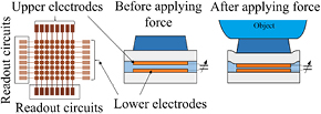
Figure 2. Working principle of the sensing unit.
Download figure:
Standard image High-resolution image3. Analytical modeling
3.1. General model
For analytical modeling, the sensing unit is simplified into a three-layer plate structure: lower PET, middle solid PDMS and upper PET films, as shown in figure 3(a). The thicknesses of the three layers are 25 μm, 20 μm and 25 μm, respectively. As shown in figure 3(a), an xyz coordinate system is defined with the origin point located at the center of the structure and z-axis perpendicular to the upper PET film. According to [25], the top PDMS bump can be replaced by applying a uniform pressure q0 on the upper PET film with an area of 3000 × 3000 μm at the center. The coordinates of the plate structure are normalized as 
 and
and  with
with ![$X,Y,Z\in \left[-1,1\right].$](https://content.cld.iop.org/journals/0960-1317/25/3/035017/revision1/jmm506709ieqn004.gif)

Figure 3. (a) Overview of the three-layer plate structure and the (b) central, (c) edge and (d) corner regions.
Download figure:
Standard image High-resolution imageSince the Young's modulus of the PET (4000 MPa) is much larger than that of the PDMS (0.55 MPa), the deformation of the PET film is much smaller than the PDMS film. This will produce strong nonlinear relation between the deformation and coordinates of the z-axis. To achieve accurate deformation prediction of the sensing unit, a nonlinear function which describes the deformation tendency along the lower PET, PDMS and upper PET films of the three-layer plate structure in the z-axis will be obtained by analyzing the deformation of the PET and PDMS films under the same pressure as detailed in appendix ![$f(Z)=[322/(1+{{\text{e}}^{-7Z-0.03}})-0.3],$](https://content.cld.iop.org/journals/0960-1317/25/3/035017/revision1/jmm506709ieqn005.gif) which is shown in equation (A.6). Using the nonlinear function, the general model of the three-layer structure can be expressed as
which is shown in equation (A.6). Using the nonlinear function, the general model of the three-layer structure can be expressed as
where u, v, w are the displacement components in the x-, y- and z-axis, respectively;  are the coefficients to be solved; i, j and k are the serial index and I, J and K are the maximal number of the serial index;
  are Chebyshev polynimials [26].
The relations between the strain and displacement are expressed in normalized coordinate as
The material properties of the sensing unit are obtained by stretching and compression tests. The Young's modulus of the PDMS with 10:1 and 20:1 are measured as 2.03 MPa and 0.55 MPa, respectively, while the PET is 4000 MPa. Accordingly, the Poisson's ratio of the PDMS with 10:1, 20:1 and PET are 0.49, 0.49 and 0.4, respectively. The Lame's first parameter λ and second parameter G [27] can be calculated as
where E and v are the Young's modulus and Poisson's ratio, respectively; ![$Z\in \left[-1,-10/35\right],$](https://content.cld.iop.org/journals/0960-1317/25/3/035017/revision1/jmm506709ieqn008.gif)
![$Z\in \left[-10/35,10/35\right],$](https://content.cld.iop.org/journals/0960-1317/25/3/035017/revision1/jmm506709ieqn009.gif) and
and ![$Z\in \left[10/35,1\right]$](https://content.cld.iop.org/journals/0960-1317/25/3/035017/revision1/jmm506709ieqn010.gif) represent the coordinate ranges in the z-axis of the lower PET, PDMS and upper PET films, respectively.
represent the coordinate ranges in the z-axis of the lower PET, PDMS and upper PET films, respectively.
Based on the Ritz method [28], the energy of the plate structure is minimized by setting the partial derivative of the energy with respect to the undetermined coefficients 
 and
and  equal to zero, so we have
where 
According to equations (1)–(4), the governing equation of this three-layer plate structure can be expressed as

where  (
( ) and Q are the stiffness sub-matrices and the loading vector, respectively.
  (
( ) are the column vectors containing undetermined coefficients of the general model in equation (1). The sub-matrices, loading vectors and column vectors in equation (5) are calculated in appendix
By substituting I = J = K = 20, q0 = 100 kPa into equations (1)–(4) and solving equation (5), the undetermined coefficients in column vectors  (
( ) are obtained and the general model in equation (1) is solved. Theoretically, setting a larger value of I, J and K will increase the accuracy because more terms of functions are utilized [28]. However, a practical limit to the number of terms that are utilized always exists because of larger truncation error when computing the stiff-matrices in equation (5) and it may generate sparse matrices that cannot be solved. These factors will reduce the accuracy and stability of the model. To accurately predict the deformation without increasing the values of I, J and K, a modified model will be developed by studying the central, edge and corner regions separately.
3.2. Modified model
The three-layer plate structure can be divided into nine regions: one central, four edges, and four corners, as in figure 3(a). Due to the symmetrical location of the four edge and corner regions, one edge and one corner region together with the central region are selected for consideration. The selected edge region locates at the negative side of the x-axis and the selected corner region locates at both negative sides of x- and y-axes, as shown in figures 3(c) and (d). The dimensions of the central, edge and corner regions are 2000 × 2000 × 70 μm, 2000 × 1000 × 70 μm and 1000 × 1000 × 70 μm, respectively. The distance between the edge of the central region and the loading region is 500 μm, which is seven times larger than the thickness of the plate (70 μm). According to the Saint–Venant theory [27], it can be inferred that the pressure in the corners and edges of the loading region will not deform the central region. Similarly, pressure in the corners of the loading region will not deform the edge region. For abbreviation, three local coordinate systems (
 and
and  ) are created for these three regions. In each local coordinate system, the origin point locates at the center and the z-axis is perpendicular to the upper PET film, as shown in figures 3(b)–(d).
In the central region, a uniform pressure q0 is applied on the upper PET film with a loading area of 2000 × 2000 μm, as shown in figure 3(b). The coordinates are normalized as 
 and
and  with
with ![${{X}_{1}},{{Y}_{1}},{{Z}_{1}}\in \left[-1,1\right].$](https://content.cld.iop.org/journals/0960-1317/25/3/035017/revision1/jmm506709ieqn027.gif) Since the uniform pressure is applied on the whole region surface, the deformation of the central region in the arbitrary plane parallel to the z1-axis is zero in the x1- and y1-axis. The bottom of the lower PET film is fixed. Thus, the displacement field function of the central region can be expressed as
Since the uniform pressure is applied on the whole region surface, the deformation of the central region in the arbitrary plane parallel to the z1-axis is zero in the x1- and y1-axis. The bottom of the lower PET film is fixed. Thus, the displacement field function of the central region can be expressed as
where  are the coefficients to be calculated.
When uniform normal force is applied, the strain of the central region is
Using the procedure described in the general model, total energy of the central region is minimized as
According to equations (3) and (6)–(8), the governing equation of the central region can be obtained as

where  and
and  are the stiffness matrix and the loading vector, respectively.
  is the column vector containing undetermined coefficients of the model in equation (6). The matrix and vectors in equation (9) are described in appendix
For the edge region, a uniform pressure q0 is applied on the upper PET film with an area of 2000 × 500 μm, as shown in figure 3(c). The coordinates can be normalized as 
 and
and  with
with ![${{X}_{2}},{{Y}_{2}},{{Z}_{2}}\in \left[-1,1\right].$](https://content.cld.iop.org/journals/0960-1317/25/3/035017/revision1/jmm506709ieqn035.gif) The bottom (
The bottom ( ) and left side (
 ) of the edge region are fixed. The right side (
 ), which is connected to the central region, has the same boundary condition as the central region. Due to the uniform pressure applied along the y2-axis being constant, the deformation in arbitrary plane perpendicular to the y2-axis is zero in the y2-axis. Thus, the boundary conditions are such that
  when
when 
 when
when  and
and  when
when  Then, the displacement field function of the edge region can be expressed as
where  and
and  are the undetermined coefficients.
According to equation (10), the strain field of the edge region is given as
Similarly, the following equations minimize the energy of the edge region as
where 
Based on equations (3) and (10)–(12), the following governing equation of the edge region is

where  (
( ) and
) and  are the stiffness sub-matrices and the loading vector, respectively.
  are the column vectors containing undetermined coefficients of the model in equation (10). The sub-matrices and vectors mentioned above are calculated in appendix
For the corner region, a uniform pressure q0 is applied with an area of 500 × 500 μm, as shown in figure 3(d). The coordinates are normalized as  with
with ![${{X}_{3}},{{Y}_{3}},{{Z}_{3}}\in \left[-1,1\right].$](https://content.cld.iop.org/journals/0960-1317/25/3/035017/revision1/jmm506709ieqn053.gif) The bottom (
The bottom ( ), left side (
 ) and back side (
 ) of the corner region are fixed. The right side (
 ) and front side (
 ) are connected to the edge region. Thus, the boundary conditions of the corner region are such that
  when
when  when
when  and
and  when
when  The displacement field function of the corner region is
where  ,
,  are the undermined coefficients.
The strain fields of the corner region are 3D functions that can be calculated as
Using the same procedure as described in the central and edge regions, the total energy of the corner region is minimized as
where 
According to equations (3) and (14)–(16), the governing equation of the corner region can be expressed as
where  and
and  are the stiffness sub-matrices and the loading vector, respectively.
  are the column vectors containing undetermined coefficients of the model in equation (14). The sub-matrices and vectors in equation (17) are calculated in appendix
By setting I = J = K = 20, q0 = 100 kPa and solving the equations (9), (13) and (17), the displacement field functions of the central, edge and corner regions can be obtained. Thus, the deformation of the sensing units can be predicted by the combination of the displacement functions which are calculated in the central, edge and corner regions.
3.3. Deformation of the sensing unit
For the developed tactile sensor, the deformations of the lower and upper electrodes (on the lower and upper PET films) need to be studied. They determine the capacitance change of the sensing unit. Here, we utilize the modified analytical model developed in the above section to study the deformations of the upper and lower PET films under uniform normal force. Figures 4(a) and (b) show the calculated deformations of the bottom surface of the upper PET film and the top surface of the lower PET film, respectively. Two cross-sections P–P' (crossing central and edge regions) and Q–Q' (crossing edge and corner regions) are created with distances of 2 mm and 0.5 mm away from the side of sensing unit, respectively. Also, figures 5(a)–(b) show the deformations in the cross-sections P–P' and Q–Q'. On the bottom surface of the upper PET film (figure 4(a)), the maximum deformation is 0.22 μm, about 600 times larger than that of the top surface of lower PET film (0.35 nm in figure 4(b)). This result is expected because the upper PET film is laminated on a soft PDMS film, thus can be deformed easily when external force applied. Therefore, when calculating the capacitance between the upper and lower electrodes, the deformation of the lower electrode could be omitted, because it has little effect on the capacitance change. Comparing figures 5(a) with (b), the deformations in cross-section P–P' are larger than those in Q–Q', because the loading area on the central region is larger than that on the edge and corner regions, as shown in figures 3(b)–(d). In figures 5(a) and (b), slight waves are observed in the edge and corner regions. When force is applied, the PDMS film in the central region will be squeezed towards the edge and corner regions and generate small waves on the edges of the loading area. Results demonstrate that the modified analytical model can accurately describe the deformation of the sensing unit.

Figure 4. Deformations of the (a) bottom surface of the upper FET film and (b) top surface of the lower PET film under uniform normal force.
Download figure:
Standard image High-resolution image
Figure 5. Predicted deformations of the upper and lower PET films at cross-sections (a) P–P' and (b) Q–Q'.
Download figure:
Standard image High-resolution imageBesides uniform normal force, uneven normal force and shear force usually occur on the sensing unit in actual applications. In this study, the uneven normal force and shear force, which can be expressed by 2D loading functions as in [25], are applied on the sensing unit. Then, the modified model is used to calculate the deformations of the sensing unit under uneven normal force and shear force. The calculation procedures are the same as those described in section 3.2 by replacing the uniform normal force q0 with the uneven normal force and shear force loading functions, respectively. Figures 6(a) and 7(a) show the calculated deformations of the upper PET film under uneven normal force and shear force, respectively. For the applied uneven normal force, the upper PET film will generate uneven deformation. For comparison, the deformations at the cross-section P–P' of the upper PET film when applying uniform and uneven normal forces with the same magnitude are shown in figure 6(b). The applied uneven normal force generates much greater deformation at the central region. For the applied shear force, the upper PET film is stretched on the negative x-axis side and is compressed on the other side, as shown in figure 7(b). The deformation predictions by the modified model are the same as the results obtained in [25]. According to the calculated deformations in figures 6 and 7, the percentage capacitance changes under uneven normal force and shear force can be calculated as 1.06% and 0.04%, respectively, while the uniform normal force causes 0.98% capacitance change. Results demonstrate that the uneven normal force, compared with uniform normal force, will generate greater capacitance change and that the sensing unit is not sensitive to shear force.
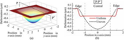
Figure 6. (a) Deformation of the upper PET film under uneven normal force and (b) P–P' cross-section view.
Download figure:
Standard image High-resolution image
Figure 7. (a) Deformation of the upper PET film under shear force and (b) P–P' cross-section view.
Download figure:
Standard image High-resolution image4. Experimental validation
4.1. Fabrication process
Figures 8(a)–(d) shows the fabrication process of the flexible capacitive tactile sensor array. To enhance sensitivity, a softer PDMS (Sylgard 184, A:B = 20:1 in weight) is used to make the dielectric layer, while the bump is made of harder PDMS (Sylgard 184, A:B = 10:1 in weight). For the fabrication of the electrode layer, a 25 μm-thick PET film is firstly adhered to a 3 inch silicon wafer, as shown in figure 8(a). Then, Cu electrodes are magnetron sputtered on the PET film. PDMS (20:1) is spin-coated on the electrodes at 7000 rpm for 40 s to form a 10 μm-thick PDMS film. The PDMS film is cured at room temperature for 24 h to generate the electrode layer. To form a capacitor, two electrode layers are fabricated with the PDMS surface activated by the oxygen plasma. Then, these two electrode layers are positioned and bonded, forming a capacitive layer, as shown in figure 8(b).

Figure 8. Fabrication process of capacitive tactile sensor array: (a) electrode layer, (b) capacitive layer, (c) PDMS bump and (d) final fabricated sensor array.
Download figure:
Standard image High-resolution imageFigure 8(c) shows the process of fabricating the PDMS bump. The liquid-state PDMS (10:1) is casted and cured at 80 °C for 3 h in a stainless steel mold, which is manufactured by electrical discharge machining (EDM), to replicate the shape of the bump and generate a PDMS mold. After peeling off, the PDMS mold is treated by the release agent (mixture of ethanol and detergent) for 30 min. Then, the liquid-state PDMS (10:1) is casted into the PDMS mold and laminated by the fabricated capacitive layer. The PDMS bump is cured at room temperature for 24 h and then peeled off from the PDMS mold together with the fabricated capacitive layer. The final capacitive tactile sensor array is shown in figure 8(d).
Figure 9(a) shows the fabricated capacitive tactile sensor array, which has 64 sensing units. The overall dimensions for the sensor array are 35 × 35 mm. Figure 9(b) shows the close-up view of the sensing units; the spatial resolution of the sensor array is 4 mm. The sensor array features high flexibility, as shown in figure 9(c).

Figure 9. (a) The fabricated capacitive tactile sensor array with 8 × 8 sensing units, (b) close-up view of the sensor array and (c) illustration of high flexibility.
Download figure:
Standard image High-resolution image4.2. Experimental setup and procedure
To study the sensing performance of the sensor array, experiments have been conducted. Figure 10(a) shows the overall experimental setup. The sensor array is placed on an electronic balance, which has 0.01 g resolution and 2000 g measurement range. A round loading bar with diameter of 4 mm is fixed onto a three-axis positioner (Newport M460P) to apply forces on the PDMS bump of the sensing unit, as shown in figure 10(b). The applied force will be measured by the electronic balance and the corresponding capacitance change of the sensing unit is measured by a LCR meter (Applent AT2818), which has a resolution of 0.01 fF and measurement range of 1 F.

Figure 10. (a) Experimental setup for the sensor array and (b) close-up view of the contact between the loading bar and PDMS bump.
Download figure:
Standard image High-resolution imageExperiment procedures are as follows: (1) Initial capacitances of the sensor array are measured, without the loading bar contacting with the sensing unit; (2) For each sensing unit, 0 to 10 N force is applied by the loading bar and the capacitance changes are recorded by the LCR meter. For each sensing unit, three repeated tests have been conducted.
4.3. Results and discussion
Figure 11(a) shows the measured initial capacitances of all the 64 sensing units. The average and standard derivation of the initial capacitances are 10.64 ± 1.03 pF. The minimum and maximum capacitances are 7.82 pF (row 2, column 3) and 12.63 pF (row 8, column 5), respectively. Figure 11(b) shows the measured percentage capacitance changes versus applied normal forces of the sensing unit (at row 3, column 6). C and C0 are the capacitance induced by the applied force and initial capacitance, respectively. The upper and lower bounds of the error bars present the maximum and minimum of the measured percentage capacitance changes. A least squares linear curve fits the experiment data, as shown in figure 11(b). The slope of the fitted line (1.24%/N) represents the sensitivity of this sensing unit.

Figure 11. (a) Initial capacitances of the sensor array and (b) capacitance changes versus forces of the sensing unit at row 3, column 6.
Download figure:
Standard image High-resolution imageBy using the same method, the sensitivities of all the 64 sensing units are obtained, as shown in figure 12. The sensitivities vary from 1.19 to 1.26%/N and the average and standard derivation of the sensitivities are 1.24 ± 0.01%/N. Table 1 summarizes the measured initial capacitances and experimental fitted sensitivities of the 64 sensing units.

Figure 12. Measured sensitivities of 64 sensing units for the sensor array.
Download figure:
Standard image High-resolution imageTable 1. Initial capacitances, sensitivities and errors of the sensing units.
| 1 | 2 | 3 | 4 | 5 | 6 | 7 | 8 | ||
|---|---|---|---|---|---|---|---|---|---|
| 1 | Ini. cap. (pF) | 9.76 | 9.74 | 10.56 | 10.54 | 10.87 | 10.64 | 10.65 | 10.63 |
| Sensitivity (%/N) | 1.245 | 1.251 | 1.259 | 1.253 | 1.245 | 1.242 | 1.244 | 1.257 | |
| Err. of sens. (%) | 0.4 | 0.08 | 0.72 | 0.24 | 0.4 | 0.64 | 0.48 | 0.56 | |
| 2 | Ini. cap. (pF) | 8.45 | 8.24 | 7.82 | 9.15 | 10.77 | 11.66 | 11.14 | 10.65 |
| Sensitivity (%/N) | 1.239 | 1.255 | 1.247 | 1.256 | 1.260 | 1.242 | 1.249 | 1.252 | |
| Err. of sens. (%) | 0.88 | 0.4 | 0.24 | 0.48 | 0.8 | 0.64 | 0.08 | 0.16 | |
| 3 | Ini. cap. (pF) | 9.35 | 9.40 | 10.07 | 9.59 | 10.13 | 10.30 | 9.62 | 9.76 |
| Sensitivity (%/N) | 1.241 | 1.241 | 1.215 | 1.246 | 1.240 | 1.254 | 1.257 | 1.235 | |
| Err. of sens. (%) | 0.72 | 0.72 | 2.8 | 0.32 | 0.8 | 0.32 | 0.56 | 1.2 | |
| 4 | Ini. cap. (pF) | 9.49 | 10.01 | 9.65 | 9.68 | 10.40 | 10.52 | 9.95 | 9.95 |
| Sensitivity (%/N) | 1.252 | 1.254 | 1.254 | 1.189 | 1.250 | 1.253 | 1.245 | 1.242 | |
| Err. of sens. (%) | 0.16 | 0.32 | 0.32 | 4.88 | 0 | 0.24 | 0.4 | 0.64 | |
| 5 | Ini. cap. (pF) | 9.47 | 9.95 | 10.67 | 10.94 | 11.09 | 10.93 | 10.33 | 10.49 |
| Sensitivity (%/N) | 1.249 | 1.257 | 1.250 | 1.244 | 1.247 | 1.257 | 1.241 | 1.245 | |
| Err. of sens. (%) | 0.08 | 0.56 | 0 | 0.48 | 0.24 | 0.56 | 0.72 | 0.4 | |
| 6 | Ini. cap. (pF) | 11.22 | 11.64 | 11.43 | 11.15 | 11.55 | 11.28 | 11.63 | 11.28 |
| Sensitivity (%/N) | 1.242 | 1.244 | 1.255 | 1.252 | 1.242 | 1.251 | 1.240 | 1.239 | |
| Err. of sens. (%) | 0.64 | 0.48 | 0.4 | 0.16 | 0.64 | 0.08 | 0.8 | 0.88 | |
| 7 | Ini. cap. (pF) | 10.92 | 10.92 | 11.12 | 11.61 | 12.04 | 11.70 | 10.60 | 11.29 |
| Sensitivity (%/N) | 1.259 | 1.239 | 1.244 | 1.242 | 1.249 | 1.258 | 1.253 | 1.246 | |
| Err. of sens. (%) | 0.72 | 0.88 | 0.48 | 0.64 | 0.08 | 0.64 | 0.24 | 0.32 | |
| 8 | Ini. cap. (pF) | 11.03 | 12.36 | 12.20 | 12.03 | 12.63 | 12.34 | 12.35 | 11.99 |
| Sensitivity (%/N) | 1.256 | 1.253 | 1.245 | 1.250 | 1.240 | 1.244 | 1.260 | 1.247 | |
| Err. of sens. (%) | 0.48 | 0.24 | 0.4 | 0 | 0.8 | 0.48 | 0.8 | 0.24 | |
To verify the developed models, the capacitance of the sensing unit is calculated using the general model (equation (1)) and the modified model (equations (6), (10) and (14)). The deformation of the bottom surface of the upper PET film can be calculated as

where F is the applied normal force ranging from 0 to 10 N,  and
and  are the deformations induced by F and q0, respectively;
  mm2 and
  kPa.
kPa.
Then, the capacitance of the sensing unit can be calculated as
where  is relative permittivity of the PDMS film [29] and k = 9.0 × 10⁹ is static electricity constant.
By setting  in equation (19), the initial capacitance of the sensing unit can be easily calculated as 10.66 pF, which is almost consistent with the measured average initial capacitance (10.64 pF). According to equations (18)–(19), the general model and modified model are utilized to calculate the capacitance change of the sensing unit and then compared to the experiment data, as shown in figure 11(b). It can be seen that the modified model can accurately predict the capacitance changes compared with the general model. For the sensing unit located at row 3, column 6, the predicted sensitivities by the general and modified models are 1.05%/N and 1.25%/N, respectively. The discrepancy between the predicted sensitivities by general model and experimental measurement are 15.3%, which is much larger than the discrepancy (0.8%) between the modified model and experiment. Results demonstrate that the modified model can accurately predict the sensitivity of the sensing unit at row 3, column 6. Also, the discrepancies of the sensitivities between the modified model predicted and experimental measurements are summarized in table 1. The maximum error is 4.88% which occurs at column 4, row 4. For all the 64 sensing units, the average error is only 0.56%. High accuracy demonstrates that the developed modified model can accurately predict the capacitance change and sensitivity of all the sensing units for normal force measurement.
For the tactile sensor array, the adjacent units will inevitably be affected when applying force on a sensing unit. We apply a 5.21 N normal force on the sensing unit U44 (at row 4, column 4) and then measure the capacitance changes of this sensing unit and its adjacent units. Experiment measurement shows that the capacitance of U44 increased from 9.68 to 10.27 pF, about 6.1% capacitance change. The capacitances of its eight adjacent units decrease in the range of 0.015%–0.019%. The result demonstrates that the interactions between adjacent units are small. The gap between two adjacent units is 1000 μm, about 18.2 times larger than the thickness of the upper PET and PDMS film (55 μm in total). Thus, according to the Saint–Venant theory [27], the loading force applied on one sensing unit will have little effect on its adjacent units.
The sensing performance of the sensor array mounted on a curved surface with 30 mm radius of curvature has been studied, as shown in figure 13. The average initial capacitances of the sensing units increase 0.35% compared to those on the flat surface. When the sensor array is bent onto a curved surface, the dielectric layer is compressed, which leads to the capacitance increase. Since the un-patterned PDMS film has been utilized as the dielectric layer, it will not be compressed too much during bending. Thus, the capacitance increase is small (0.35%). Then, we apply 0–10 N normal force on the sensing unit U44 (at row 4, column 4) and the capacitance change is measured as 15.1% when the force is 10 N. The capacitance change calculated by the modified model is 12.5%. The discrepancy between the measured and calculated results is 2.6%. When the sensor has been mounted onto the curved surface, the bump surface will also be bent into a curved shape. The loading bar, which contacts with the curved bump surface, will induce uneven force on the sensing unit and thus generates larger capacitance increase, as described in section 3.3. As the radius of curvature of the curved surface decreases, the contact force on the sensing unit becomes more uneven, thus the accuracy of the modified model will be decreased. For accurate prediction of the capacitance change, the effects of the curved surface need to be considered and incorporated into the developed models, which has become our future work.

Figure 13. The percentage capacitance change of the sensing unit U44 when the sensor array is mounted onto a curved surface.
Download figure:
Standard image High-resolution image
5. Conclusions
We have developed a modified analytical model, based on the Ritz method, to study the sensing performance of the sensing unit for flexible capacitive tactile sensor array. By dividing the sensing unit into the central, edge and corner regions, the modified model is established and can accurately predict the deformation of the sensing units. For validation, we have fabricated a capacitive sensor array with 64 sensing units and the average initial capacitance and sensitivity is 10.64 pF and 1.24%/N, respectively. The developed modified model is used to predict the capacitance change and sensitivity of the sensor array with the value of 1.25%/N. High accuracy demonstrates that the modified model can accurately predict the sensing performance of the sensor array. Future work will focus on the structural optimization of the tactile sensor array by using the established analytical model to reduce the discrepancies caused by the uneven and/or shear forces.
Acknowledgments
The authors would like to acknowledge the support from the National Basic Research Program (973) of China under Grant No. 2011CB013300, National Natural Science Foundation of China under Grant Nos. 51105333 and 51275466 and Science Fund for Creative Research Groups of National Natural Science Foundation of China under Grant 51221004, and the Scientific Research Foundation for Returned Overseas Chinese Scholars under Grant No. 2014 1685.
Appendix A.: Nonlinear function for the general and modified models
For an infinite single-layer plate applied an infinite uniform pressure, the deformation can be calculated by simplifying the equation of equilibrium in terms of displacement [27] into a 1 D equation as
where z' is defined as the thickness direction, w' is the displacement component in the z'-axis and v is Poisson's ratio.
The stress applied on infinite plate is given by

where E is Young's modulus and v is Poisson's ratio.
By solving equations (A.1)–(A.2), the displacement field function of infinite single-layer plate can be expressed as

The PDMS (20:1) has Young's modulus of 0.55 MPa and Poisson's ratio of 0.49, while the PET has Young's modulus of 4000 MPa and Poisson's ratio of 0.4. The ratio of deformations of the PDMS film to the PET film in the z'-axis under the same pressure can be calculated by equation (A.3) as follows:
where  and
and  are the deformations of PDMS film and PET film in the z'-axis, respectively.
Since the large differences of Young's modulus between the PET and PDMS films of the sensing unit, the deformations of the PET and PDMS films in the z-axis differ largely. To achieve accurate prediction of the deformation of the sensing unit, a segmental function is defined to describe the tendency of the deformations along the z-axis by equation (A.4) as
where ![$Z\in \left[-1,-10/35\right],Z\in \left[-10/35,10/35\right]$](https://content.cld.iop.org/journals/0960-1317/25/3/035017/revision1/jmm506709ieqn078.gif) , and Z ∈ [10/35, 1] represent the lower PET, PDMS and upper PET films, respectively.
, and Z ∈ [10/35, 1] represent the lower PET, PDMS and upper PET films, respectively.
Equation (A.5) is then fitted by an S-shape function using the least square method as
Equation (A.6) describes the nonlinear relation between the deformation and coordinate in the z-axis (defined in figure 3(a)). This function can be utilized in the general and modified models to achieve more accurate deformation prediction of the proposed sensing unit.
Appendix B.: Calculation of the elements in the governing equations
B1. Calculation of the elements in the governing equations of the general model
By defining  as the element in
  th row and ijkth column, the elements of the stiffness sub-matrices in equation (5) are calculated as
in which
where 
The elements of the loading vector Q in equation (5) can be calculated as
where  is the element in kth row of the matrix Q.
The explicit form of the undetermined vector  in equation (5) is:
where 
B2. Calculation of the elements in the governing equations of the modified model
By defining  as the element in
  th row and ijk th column, the elements of the stiffness matrix in equation (9) can be calculated as
The elements of the loading vector  in equation (9) are calculated as

where  is the element in kth row of the matrix
The explicit form of the undetermined vectors in equation (9) is
By defining  as the element in
  th row and ijk th column, the elements of the stiffness matrices in equation (13) can be calculated as
The elements of the loading vector  in equation (13) are calculated as

where  is the ijkth element of the matrix
The explicit form of the undetermined vectors in equation (13) is:
where 
By defining  as the element in
  th row and ijkth column, the elements of the stiffness matrices in equation (17) can be calculated as
in which
where 
The elements of the loading vector  in equation (17) are calculated as
where  is the ijkth element of the matrix
The explicit form of the undetermined vector in equation (17) is
where 