

Abstract
In the aeronautical industry, composite structures under testing often have complex and variable geometries. In such cases, an optimal use of ultrasonic transducer arrays requires specific algorithms in electronic systems in order to achieve rapid and reliable inspections. To fulfil such requirements, a new real-time and adaptive technique is presented. The surface adaptive ultrasound (SAUL) technique is based on an iterative algorithm that does not require a prior knowledge of the geometrical properties of the inspected domain. All different parts of a given component can be controlled using the same transducer array, such as a conventional linear array with a flat shape. In this paper, the adaptive processing is demonstrated through acquisitions performed with different typical aircraft composite structures. In addition, we present a new surface reconstruction algorithm. This fast algorithm is efficient and can be coupled with the real-time adaptive processing to reconstruct SAUL images and, then, to improve the characterization of flaws in composite materials.
Export citation and abstract BibTeX RIS
1. Introduction
New commercial aircraft models incorporate more and more composite materials in their structures to ensure both lightness and robustness. This increase in composite surfaces motivates the development of new technologies and algorithms in ultrasonic nondestructive testing (NDT) to achieve fast and reliable inspections. Ultrasonic transducer arrays represent the most promising technological solution to reduce scanning times and to also improve the characterization of defects. In general, these sensors are used to detect manufacturing defects (porosities, foreign bodies, delaminations, cracks, etc) introduced in composite materials during manufacturing processes [1].
One of the most famous acquisition modes is the so-called paintbrush acquisition. It consists in transmitting simultaneously with all the elements of a phased array, without a delay law, and in receiving the individual signals in parallel with all the elements [2, 3]. This mode leads to high scanning speeds that do not depend on the number of elements used. In order to improve the signal to noise ratio, a sub-aperture of few consecutive elements can be used in reception. This sub-aperture is moved all along the total aperture and the elementary signals are summed at each electronic step.
For complex geometries, such as the curved parts of aeronautical stiffeners or stringers, a solution consists in using shaped probes, such as cylindrical transducer arrays. The probe is placed over the convex surface and its curvature radius ensures a normal incidence transmission of the ultrasonic field at any point of the surface [4, 5]. Inspection is performed by mechanically adjusting the lateral position during scanning to master the normal incidence transmission. The main drawback of shaped probes is that they are only valid for one type of geometry and that they require a high-precision positioning device in order to be accurate. In addition, other parts of a given component may require a large inventory of probes with different shapes, which leads to expensive NDT costs and reduces inspection speeds when a complex part has to be inspected in its entire totality.
In this paper, a self-adaptive ultrasonic method is presented. The technique allows us to master a normal incidence transmission through various complex surfaces using a conventional non-shaped phased array (typically a linear or matrix array with a flat active aperture). A given component presenting variable geometries can be fully inspected with the same probe. This is achieved by means of an iterative algorithm, which is a generalization of the one described in [2] and used in [6, 7]. The basic principle consists in measuring times of flight from a surface echo recorded in paintbrush mode and in deducing an adaptive delay law exciting an incident wave front parallel to the surface [8]. The self-adaptive technique is called the SAUL method (acronym for 'surface adaptive ultrasound') and has been implemented in the multichannel MultiX systems, designed by the M2M Company. The real-time processing is first described and then validated with measurements performed on different carbon fiber reinforced plastic (CFRP) aeronautical structures.
Currently, the MultiX systems do not allow the full characterization of a flaw accuracy (e.g., its size and depth) because the exact geometry and/or the position of the corner radius (e.g., the scanning axis is not exactly parallel to the corner radius one) are not assumed to be known during inspection. The SAUL processing is an efficient adaptive detection technique but the surface geometry must be reconstructed in real-time to make images and improve the flaw characterization.
In order to reconstruct images with the SAUL technique, we suggest a fast surface reconstruction algorithm introduced for radar systems and based on the computation of an envelope of circles or spheres [9–11]. The simplicity and robustness of the algorithm are suitable for real-time operations. Compared to the previous works in electromagnetics where quasi point-like sources are assumed, the originality of our approach lies in the fact that the reconstruction algorithm is applied to a large array, where all the elements are excited at the same time with a delay law provided by the SAUL algorithm. This approach is interesting for very fast inspections since only a few ultrasonic shots are needed to reconstruct the whole surface geometry in front of the array. Indeed, the reconstruction speed does not depend on the number of array elements but on the number of iterations in the SAUL processing.
2. Principle of the SAUL method
2.1. Paintbrush acquisition mode
The experimental set-up used throughout the paper is described in figure 1. It consists in a MultiX parallel acquisition system with 128 channels, and a computer that drives both the system and a linear motorized positioning system to set the probe position. The part under testing is an aeronautical CFRP stringer and the main objective is to control its curved part, also called 'corner radius'. The thickness and the length of the composite are 5 and 380 mm, respectively, and the curvature radius of the front interface is approximately 14 mm (this curvature radius is not rigorously constant along the corner radius). The probe is a linear transducer array (with a central frequency of 5 MHz) composed of 128 elements of 0.5 × 8 mm2, with 0.6 mm pitch. In practice, only 42 active elements are used in this section to inspect the curved part of the component. This probe is immersed in the tank over the convex surface, with a water path of 16 mm. Note that, in this section, the SAUL method is introduced for a fixed position of the probe. Real-time results will be presented in the next section by translating the transducer array along the corner radius.
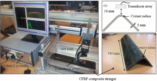
Figure 1. Experimental set-up including a parallel acquisition system with 128 channels, a computer driving the system, and a composite corner radius immersed in a tank (a). A linear transducer array is immersed in the tank and positioned in front of the convex surface of the corner radius (b)–(c).
Download figure:
Standard image High-resolution imageThe paintbrush acquisition mode consists in transmitting a plane wave by firing with the full array and in recording the elementary signals in parallel with all the elements. The experimental Bscan-channels image (channels/time) acquired with the MultiX system is displayed in figure 2(a) (no electronic scanning has been used in reception). We can observe the front surface echo between 22 and 24 µs (see the time of flight curve in figure 2(b)), while the back surface echo is not visible. Since the incident wave is not in the direction normal to the surface, the successive plies inside the material (each ply being approximately parallel to the surface) refract the transmitted field during its propagation and practically almost no energy reaches the back surface. This results in a poor image where both the plies and the back interface of the corner radius can not be identified.

Figure 2. Bscan image obtained in paintbrush acquisition mode (a) and time of flight curve (b).
Download figure:
Standard image High-resolution image2.2. Principle for adapting a wave to a complex surface
The incident wave can be partially adapted to the surface according to the processing described in [2] and [6, 7]. First, the times of flight between all the elements of the array and the surface are measured (for instance, by detecting the maxima of the surface echo envelope). Then, these times of flight are used to extract a delay law that will be applied to a second shot. Denoting by ti the time of flight between an element i and the surface (1 ≤ i ≤ 42), the transmission delay applied to this element is defined by

A reception delay law can also be applied in order to synchronize each received signal and, for instance, to create several coherent summations of signals using an electronic scanning of a sub-aperture. The reception delay applied to an element i is deduced from the transmission delays as follows:

By applying the transmission and reception adaptive delay laws to the second ultrasonic shot, the new Bscan image in figure 3(a) is obtained. The delay laws are displayed in figure 4(a) and are deduced from the times of flight plotted in figure 2(b). Compared to the first acquisition, the back surface echo can now be identified, which confirms that the delay law calculated with (1) transmits the incident wave with a wave front almost parallel to the front surface. The anisotropy effects due to the fibrous nature of the material are minimized by forcing a normal incidence transmission. However, as the incident wave is not completely adapted to the front surface, the back surface echo has a low amplitude level and the internal composite structure still can not be identified (the plies are not clearly visible). In addition, the elementary signals are not accurately synchronized, which could result in a poor image if an electronic scanning with a sub-aperture of several elements was used in reception.
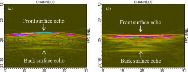
Figure 3. Bscan images obtained when adaptive delay laws are deduced from a paintbrush acquisition (a) and from an electronic scanning in transmission (b).
Download figure:
Standard image High-resolution image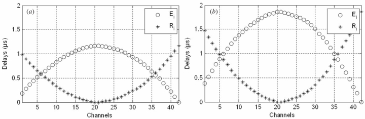
Figure 4. Delay laws deduced from a paintbrush acquisition (a) and from an electronic scanning in transmission (b).
Download figure:
Standard image High-resolution imageFor a geometry as complex as a corner radius, the incident wave is not perfectly adapted to the surface since the times of flight used in the delay law computation are not specular (a specular time of flight corresponds to the path along the ray passing through the center of an element and normal to the surface). A technique for measuring these specular times of flight consists in using an electronic scanning in transmission with a sub-aperture and a scanning step of 1 element (all the elements are excited separately, and the same element is used as transmitter and receiver for each shot).
Figure 4(b) shows the new delay laws, obtained with the same experimental set-up. The only difference lies in the times of flight that now correspond to specular paths. Their measurement requires a cycle of 42 shots since the transducer array is composed of 42 active elements. Next, these delay laws are applied to one last shot (transmission once with all the elements). In figure 3(b), one can see that the individual signals are now time coherent (the front surface echo is horizontal), which means that the incident wave is ideally adapted to the geometry. The ply echoes now can be observed.
This method thus provides the optimal delay laws to achieve a normal incidence transmission into the material. However, in its current state, it can not be applied to industrial controls for two reasons. First, since a single element is used at each transmission, the amplitude level of the surface echo is much lower than the one obtained by transmitting with the full array and times of flight may be difficult to be measured. Second, the large number of shots (43 in the present case) may dramatically decrease inspection rates compared to a conventional paintbrush acquisition mode.
2.3. The surface adaptive ultrasound algorithm
The SAUL method is an iterative processing of a conventional paintbrush acquisition. The processing thus begins with the transmission of a plane wave by simultaneously firing with all elements and recording individual signals in parallel separately with the full array. As previously described, the adaptive delay laws are then calculated and used in turn for a second ultrasonic shot.
In the SAUL method, this processing is iterated as many times as necessary, until the incident wave ideally fits the front surface, i.e. new delays laws are calculated after the second shot and are added to the previous ones; then, the resulting delay laws are applied to a third shot; and so on, until the iterative processing converges. Mathematically, the transmission delay applied to an element i (with 1 ≤ i ≤ 42) is calculated as follows:


where j (j = 1, 2,...) denotes the shot number in the iterative processing (j = 1 corresponds to the first transmission without delay law, i.e.  for j = 0 ∀i). Equation (3) refers to an accumulation of delay laws after each iteration, while (4) is an offset correction ensuring that the minimum delay in the accumulated delay law is still zero. In reception, the delays are such that

For an optimal implementation in electronic systems, it is more convenient to express  and
and  only with delays related to the previous shot j. Substitution of (4) into (3) yields to the following expression for the emission delays:

Next, substituting (6) into (4), the reception delays may be expressed as

Equations (6) and (7) are the ones implemented in the MultiX systems in order to optimize inspection rates. The application of the first four transmission and reception delay laws ( and
and  with 1 ≤ j ≤ 4) in the iterative processing leads to the Bscans images in figure 5. The experimental set-up is unchanged compared to the previous part.

Figure 5. Successive Bscan images recorded in the iterative SAUL processing.
Download figure:
Standard image High-resolution imageThe set of Bscans in figure 5 illustrates the gradual adaptation of the incident wave to the front surface of the corner radius. Iteration after iteration, the amplitude levels of the front and back surface echoes gradually increase in amplitude, and the received elementary signals progressively become time coherent. At the convergence, the Bscan is identical to the one provided by an electronic scanning in transmission (see figure 3(b)). Note that, in the present case, no delay law is applied to the first shot because we assumed that no information was available about the geometry of the surface. In contrast, if rough information is available about the geometry, a non-zero delay law can be applied at the first shot in order to partially adapt the incident wave to the surface. Thus, the algorithm requires fewer iterations to converge.
2.4. Simulation of the transmitted field at each iteration
The convergence of the SAUL algorithm is demonstrated in figure 6 through simulations performed with the CIVA software platform [12]. These simulations have been simplified by considering a homogeneous and isotropic material (with the same acoustical properties as the epoxy) and by taking into account the propagation of compression waves only. In the simulation model, the interaction of waves with the component boundaries is based on the high-frequency Kirchhoff approximation, while the field propagation is governed by the semi-analytical 'pencil method' [13]. As in the experiment, the delay laws are deduced from times of flight measured from the front surface echo, but this echo is now simulated. In the CIVA model, the configuration (geometry of the component, properties of the transducer array, water path) is identical to the experimental one.
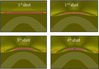
Figure 6. Simulated incident field for each iteration of the SAUL processing.
Download figure:
Standard image High-resolution imageThe simulated incident fields in figure 6 show the evolution of the incident wave front at each shot of the SAUL processing, just before the wave reaches the surface. As expected, the wave progressively fits the surface. At the fourth shot, the incident wave front has the same curvature as the front surface.
3. Real-time SAUL processing
3.1. Robustness of the adaptive processing for different geometries
Generally, the SAUL algorithm allows us to master a normal incidence transmission through any complex surface using a small number of ultrasonic shots (generally, no more than four or five shots are needed). In order to illustrate this, a second experimental set-up is considered in figure 7.
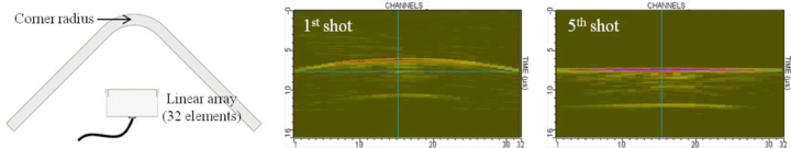
Figure 7. Linear transducer array in front of the concave surface of a corner radius with 5 mm thickness: the SAUL processing converges at the fifth shot.
Download figure:
Standard image High-resolution imageA linear transducer array (the probe is the same than previously but ten elements are disabled) is placed in front of the concave surface of the corner radius presented in figure 1. This type of geometry is the most unfavorable (because the curvature radius is smaller than the one of the convex surface and reflections on the flat surfaces may also affect the time of flight measurement) but the algorithm is robust and requires only one additional iteration to converge. Both results in figures 5 and 7 are interesting since they demonstrate that it is possible to control the concave and convex surfaces of a given composite radius using a same conventional non-shaped transducer array.
The third and last example in figure 8 is a composite stiffener with a shoulder geometry; this particular geometry includes both concave and convex surfaces with local curvature radii of 20 mm (for the convex surface) and 5 mm (for the concave one). A linear probe (with 128 elements, 10 MHz central frequency and 0.35 mm pitch) is placed in front of the complex part (its thickness is 3 mm). For this kind of geometry, the algorithm still converges quickly, at the fourth shot.
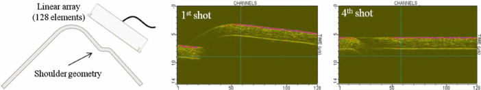
Figure 8. Linear transducer array in front of the shoulder geometry of a composite stiffener with 3 mm thickness: the SAUL processing converges at the fourth shot.
Download figure:
Standard image High-resolution imageIn order to demonstrate the robustness of the adaptive method to a lateral misalignment during scanning, figure 9 displays several screenshots of the real-time processing when a linear transducer array (the same probe used for the shoulder geometry) is translated perpendicularly to the axis of a corner radius (the one described in figure 1). The screenshots are presented for five positions of the probe, from x = −15 mm to x = 15 mm, around the top (x = 0) of the corner radius.
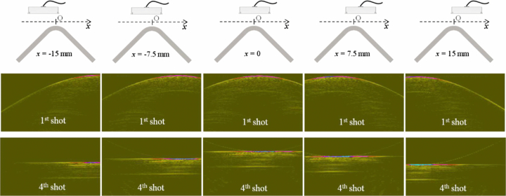
Figure 9. SAUL processing when a linear transducer array is translated perpendicularly to a corner radius: the Bscans are displayed before (top images) and after (bottom images) the SAUL processing.
Download figure:
Standard image High-resolution imageThe successive images in figure 9 clearly demonstrate the ability of the real-time processing to adapt itself to significant changes in the geometry, such as the presence of a misalignment between a probe and a corner radius. Even for very eccentric positions of the probe, figure 9 shows that the front and back surface echoes remain horizontal and that the maximum amplitude of the back surface echo is practically unchanged.
In conclusion of this part, it is important to note that the SAUL algorithm is unchanged for matrix probes and does not require specific changes in the hardware design of the MultiX systems.
3.2. Example of real-time inspection
The SAUL hardware design in the MultiX systems enables real-time inspections at high speed: using a transducer array of 48 elements and five shots in each cycle of iterations, the processing can be enabled with a frame rate of around 500 fps. It is important to note that no convergence criterion has been implemented in the hardware design. The number of iterations is constant during scanning and it is specified at the initial position of the probe. As shown above, a cycle of five shots is sufficient for most geometries encountered in aerospace.
The experimental set-up considered in this paragraph is the one described in figure 1. Two acquisitions were performed by translating the transducer over a distance of 280 mm (the initial scanning position is 40 mm from one end of corner radius) and data were recorded in 2 mm steps at a speed of 100 mm s–1. An artificial defect (a flat bottom hole with 4 mm diameter and 2 mm depth) was drilled on the concave surface (under the corner radius). It is located at mid-length of the component, at 190 mm from either end (the length of the corner radius is 380 mm). In figure 10(b), the SAUL processing was applied by using a cycle of four shots at each position, while no processing was applied in figure 10(a). In both cases, an electric scanning with a sub-aperture of four adjacent elements and a scanning step of one element was used in reception (which corresponds to 45 sequences in reception). For each scanning step, the mean of four elementary signals was calculated and represented in the form of an electronic Bscan (sequence/time).
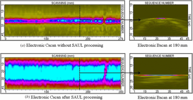
Figure 10. Electronic Cscan without processing (a) and processed with the SAUL technique with four shots in each cycle of iterations (b).
Download figure:
Standard image High-resolution imageEach electronic Cscan (position/sequence) in figure 10 results from the concatenation of the electronic Bscans recorded at each acquisition step. The comparison of the two Cscans reveals a larger surface echo when the SAUL processing is enabled. This is mainly due to the time coherence of the elementary signals rather than an increase in their amplitude. This surface echo is large enough to enable triggering during scanning and eliminate water path variations. A triggering is essential in order to set an acquisition time window at a given inspection depth below the surface, and to eliminate the surface echo that could hide an echo of interest, such as in figure 10(b).
The SAUL acquisition mode, coupled with a compensation of water path variations, can be better understood with the mechanical Bscans (position/time) displayed in figure 11. Each one represents the evolution of a single sequence (i.e. the average of four received elementary signals at the 19th sequence) as a function of the probe position. By using the SAUL processing without triggering (comparison of figures 11(a) and (b)), we note that the surface echo is much stronger and the defect echo is identified at 150 mm from the initial scanning position. However, the SAUL mechanical Bscan shows that the arrival time of the surface echo varies due to a slight misalignment between the scanning axis and the corner radius one. After triggering, in figure 11(c), the water path variations are corrected so that a 2 µs time window at 3 µs after the surface echo (corresponding to an inspection depth of around 4 mm) can be set in order to image the defect with a Cscan representation.
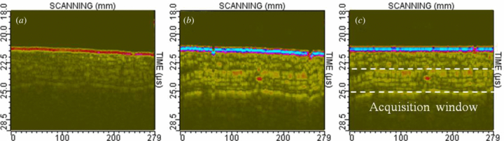
Figure 11. Mechanical Bscans displayed for the 19th sequence: initial Bscan without processing (a), Bscan with the SAUL processing (b), and SAUL Bscan with a correction of water path variations (c). A 2 µs acquisition time window is fixed at 3 µs after the surface echo.
Download figure:
Standard image High-resolution imageThe real-time SAUL processing, associated with a correction of water path variations, provides the new electronic Cscan displayed in figure 12. The artificial defect is detected with a suitable signal-to-noise ratio (around 12 dB) at 150 mm. Thus, this experimental result clearly demonstrates that it is possible to detect a defect without any prior accurate knowledge of the geometry and/or the position of a composite component. Nevertheless, it should be noted that the method does not allow for characterization of a defect (especially, its size) because the SAUL imaging is only a representation sequence/scanning of the measured amplitudes. A substantial improvement would be to reconstruct actual images of the inside of the component, which requires an implementation of fast surface reconstruction algorithms in the imaging MultiX systems. In the next section, we test an algorithm introduced in the field of radar systems and based on the computation of an envelope of circles.
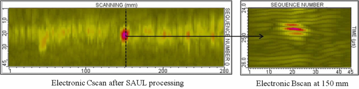
Figure 12. Electronic Cscan provided by a SAUL MultiX system: the artificial defect is detected at 150 mm from the initial scanning position.
Download figure:
Standard image High-resolution image4. Geometry reconstruction using the SAUL method
In this section, as shown in figure 13(a), the surface reconstruction algorithm will be applied to an aluminum cylinder immersed in water. Unlike the previous composite component (the geometry is slightly variable along the corner radius and the probe positioning cannot be mastered with accuracy) the geometry of the cylinder is well known, and the reconstructed surface will be compared with the theoretical one to validate the algorithm. The inner and outer radii of the cylinder are 10 and 20 mm, respectively. The probe is a linear transducer array with 128 elements (0.5 × 8 mm2, with 0.6 mm pitch) with a central frequency of 5 MHz. The water path is 15.8 mm. The SAUL processing was applied to this experimental set-up, and the Bscan (channels/time) obtained at convergence is presented in figure 13(b). The Bscan displays the outer and inner surface echoes, which are both horizontal.
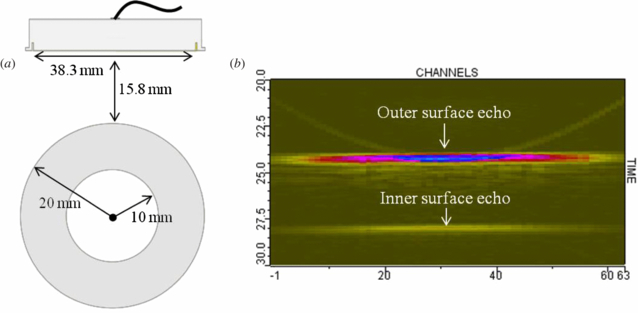
Figure 13. A linear transducer array placed above an aluminum cylinder (a) and Bscan (channels/time) obtained when the SAUL processing converges (b).
Download figure:
Standard image High-resolution imageThe reconstruction algorithm proposed in this paper is based on the computation of an envelope of circles [10, 11], and deals with the specular times of flight mentioned in section 2. These times of flight can be measured with an electronic scanning in transmission, which would require 128 shots in the present experiment (this large number of shots is not compatible with real-time operations). However, it is possible to deduce these specular times of flight from the delay laws applied in the SAUL processing. By noting Ei the transmission delay applied to an element i at convergence (the superscript '(j)' is omitted for convenience), the corresponding specular time of flight ti' (with 1 ≤ i ≤ 128) can be simply calculated as follows:

where ti is the time of flight measured from the outer surface echo in figure 13(b). This is the second interesting application of the SAUL method since, contrary to the electronic scanning method, the speed of surface reconstruction will not depend on the number of elements anymore, but on the number of iterations in the adaptive processing. In (8), it should be noted that the times of flight ti can be replaced by an average value because they are almost constant. From the specular times of flight, the surface reconstruction consists in determining the envelope of a family of circles Ci with the centers ci (i.e. the center of an element i) and radii di = v ti'/2 (where v is the phase velocity in water). With the notations introduced in figure 14, the coordinates xi and zi of each point are given by

where

For a transducer with N elements, the reconstructed profile is described by N − 1 impact points. Next, a linear interpolation can be applied to calculate the profile between two consecutive points. It is important to note that this algorithm can be easily extended to 2D matrix probes. In this case, the surface is given by the surface tangential to a family of spheres [12].
The surface reconstruction algorithm has been implemented in the CIVA software, and the post-processing of the Bscan (channel/time) in figure 13(a) provides the reconstructed profile in figure 14. The comparison with the theoretical result shows an excellent agreement: the maximum reconstruction error is less than the wavelength in water (i.e. 0.3 mm at 5 MHz). Before the reconstruction, a plane surface is considered in CIVA because the geometry is not assumed to be unknown in practice. This is why, in figure 15, the surfaces are planar on both sides of the reconstructed profile.
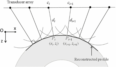
Figure 14. Geometry describing the principle of the surface reconstruction algorithm: the reconstructed profile is the curve tangential to a family of circles with the centers ci and radii di.
Download figure:
Standard image High-resolution image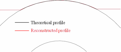
Figure 15. Superimposition of the theoretical profile (in black) and the reconstructed one (in red) of an aluminum cylinder immersed in water.
Download figure:
Standard image High-resolution image
5. Summary and conclusions
In this paper, a new adaptive inspection technique implemented in MultiX systems was presented. This technique is based on an iterative processing of a paintbrush acquisition mode and requires only a small number of ultrasonic shots to achieve a normal incidence transmission through a complex surface of a composite structure. All different parts (flat, concave or convex surfaces) of a given component can be inspected using the same ultrasonic array, such as a conventional probe with a flat active aperture. Acquisition results performed with different aircraft components were presented and showed that the SAUL method is promising in terms of scanning rate and detection ability.
Current works focus on the geometry reconstruction to improve the defect characterization. The reconstruction algorithm presented in this paper is directly applicable to a SAUL acquisition and seems to be the most suitable for high speed controls. Developments are in progress to implement this algorithm in the M2M imaging systems, especially for the 3D imaging with 2D matrix probes.
Acknowledgments
This work was supported by grants from DGCIS/CG92/CG91/IDF in the framework of the competitiveness cluster SYSTEM@TIC PARIS-REGION (CORTEX 3D project).