
Abstract
We study the microwave properties of a superconducting tunable coplanar waveguide (CPW). Pairs of Josephson junctions are forming superconducting quantum interference devices (SQUIDs), which shunt the central conductor of the CPW. The Josephson inductance of the SQUIDs is varied in the range of 0.08–0.5 nH by applying a dc magnetic field. The central conductor of the CPW contains Josephson junctions connected in series that provide extra inductances; the magnetic field controlling the SQUIDs is weak enough not to influence the inductance of the chain of the single junctions. The circuit is designed to have left- and right-handed transmission properties separated by a variable rejection band; the band edges can be tuned by the magnetic field. We present transmission measurements on CPWs based on up to 120 Nb–AlOx–Nb Josephson junctions. At zero magnetic field, we observed no rejection band in the frequency range of 8–11 GHz. When applying the magnetic field, a rejection band between 7 GHz and 9 GHz appears. The experimental data are compared with numerical simulations.
Export citation and abstract BibTeX RIS
1. Introduction
Left-handed electromagnetic materials were considered in 1967 by Veselago [1]. Using Maxwell equations, it was shown that such materials exhibit a negative index of refraction. The medium was called 'left' or 'left-handed' (LH) because the electric field E, magnetic field H and the wavevector k form a left-handed system, while in ordinary media they form a right-handed system. According to the Maxwell equations, the phase velocity of the LH media is opposite to both the direction of energy flow and the group velocity [2]. Since their first experimental realization in 2000 [3], the interest in left-handed metamaterials is unbroken and growing. One relatively simple way of implementing a left-handed medium is the building of a planar transmission line. The electric permittivity ε and magnetic permeability μ of such a transmission medium can be modeled using distributed L–C networks [4]. The traditional two-wire model of a right-handed transmission line (RHTL) with inductance L on the central conductor and capacitance C on the shunt describes an electromagnetic medium with a positive index of refraction, where L and C define positive equivalents for permeability and permittivity, respectively. A left-handed transmission line (LHTL) with negative permeability and permittivity can be created by simply exchanging the positions of L and C in the line [5].
2. Design and computer simulation
A transmission line can be described by the purely left-handed or right-handed two-wire model. However, in reality, it will always be of mixed type while LHTL or RHTL behavior can dominate within a fixed frequency range [6]. In this work, we propose, design and test a transmission line which is tunable from RHTL to LHTL under application of a dc magnetic field. The tunability of LHTLs has already been considered in some work, for example in [7, 8]. In [7], the pass-band of the line is changed by applying a dc bias current, which tunes the kinetic inductance of a superconducting wire. The tunability has been also provided via applying a static electric field to thick films of barium–strontium–titanate (BST) which changes the electrical properties of the structure.
The suggested transmission line contains dc SQUIDs as tunable elements, which are known for their high sensitivity to magnetic fields. The tuning of the dispersion is obtained by changing the Josephson inductance of the SQUIDs. Previously, Josephson junction arrays with two-junction unit cells have been studied theoretically in [9]. Here, we focus on the experimental study of a tunable rejection band in the transmission spectrum of the planar CPW. Our approach relies on the tunability of SQUIDs, which has been recently experimentally demonstrated in [10].
The Josephson inductance of the dc SQUID is given by the relation from [11]:
where Φ0 is the magnetic flux quantum, Ic is the maximum (zero field) critical current of the junction and φ is the superconducting phase difference. The phase difference defines the superconducting current through the junction in a non-zero magnetic field. It is essential to notice that the influence of the magnetic field on the inductance Lj1 of the series of Josephson junctions in the main line is negligible because the applied magnetic field is normal to the plane of the electrodes of the junction. The magnetic flux coupled to the series junctions is negligibly small, therefore the inductance Lj1 of the junctions can be assumed as a constant for the whole range of magnetic fields used in this experiment.
The lumped-element equivalent circuit of a section of our transmission line is shown in figure 1. Capacitance C1 and inductance Lj2 define the left-handed properties of the transmission line while capacitance C2 and inductance Lj1 contribute to the right-handed behavior. Since both chains C1–Lj1 and C2–Lj2 are resonators, one would expect that the line may have, depending on exact parameters of C' and L', properties of either type in different frequency bands.
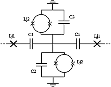
Figure 1. Scheme of a unit cell. Crosses indicate Josephson junctions, circles are SQUID loops and Lj denote the effective inductance of either SQUIDs or Josephson junctions. The experimental devices contains up to 20 cells in series, which is long enough to treat the structure as a fraction of a transmission line within the frequency range 4–12 GHz.
Download figure:
Standard image High-resolution imageIn order to understand the LHTR properties, one has to consider the dispersion relation f(β) of traveling waves as in [7]. The propagation constant β shows the phase and amplitude of electromagnetic wave along the propagation direction. An example of the frequency dependence of the propagation constant β is shown in figure 2 which is calculated for the following parameters specific to our circuit: C1 = 2.1 pF,C2 = 1.7 pF,Lj1 = 80 pH. The tunable inductance Lj2 is controlled by a small uniform dc magnetic field, which induces dissipation-free persistent currents in the loops of the SQUIDs. Figure 2(a) shows an example of the dispersion curve for Lj2 = 300 pH, while in figure 2(b) we use Lj2 = 190 pH.
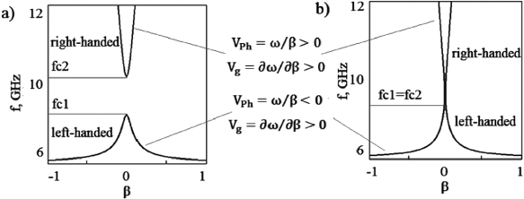
Figure 2. Calculated dispersion curves of LHTL. (a) Josephson inductance Lj2 = 300 pH leads to fc1 ≠fc2; a rejection band occurs between frequencies fc1 and fc2. (b) Josephson inductance Lj2 = 190 pH results in fc1 = fc2; the rejection band is absent.
Download figure:
Standard image High-resolution imageOne can see from figure 2 that the phase and group velocities, VPh and Vg, have opposite signs in the lower part of the dispersion spectrum. This mean that the lower transmission band is the left-handed band. In contrast, phase and group velocities have the same direction above the upper cut-off frequency, which indicates a right-handed band. The lower and upper cut-off frequencies shown in the text below are respectively the upper frequency of the left-handed band and the lower frequency of the right-handed band. These cut-off frequencies can be expressed via the following equations from [12]:
It can be seen from equations (1) and (2) that changing Lj2 one can tune the upper frequency of the rejection band.
We started our study with numerical simulation of the transmission through an array of 20 unit cells from figure 1. The results of the simulation are shown in figure 3 for different values of φ, corresponding to different values of the magnetic field. One can see that the dip in the transmission between the left-handed (lower band) and the right-handed (higher band) indeed depends on the inductance Lj2, which is controlled via application of magnetic field, as expected from equations (1) and (2). In figure 3(a) only one, the left-handed pass-band, is present. The application of magnetic field leads to the merging of the left and right-handed pass-bands as shown in figure 3(b). At even larger field cosφ gets close enough to zero, and the left-handed and right-handed bands of transmission are again separated by a rejection band. This case is depicted in figure 3(c).
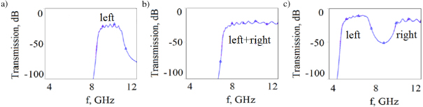
Figure 3. Simulated transmission magnitude |S21| through an array of 20 unit cells for different values of φ: (a) cosφ = 0.8, (b) cosφ = 0.4, (c) cosφ = 0.2.
Download figure:
Standard image High-resolution imageThe transmission from figure 3 does not indicate the left-handed and right-handed behavior directly. The scattering parameters (S-parameters) and the complex impedance of the cells can be used to clarify whether the band is left-handed or right-handed. Both S-parameters and impedance for the magnetic fields of figure 3(c) are depicted in figure 4. One can see from figure 4(a) that the structure demonstrates almost full reflection (S11 = 0 dB) within the frequency range of 9–11 GHz. According to figure 4(b), the edges of the reflection band coincide with the frequencies at which the imaginary part of the impedance curves, Im(Z,f), change their sign. The left-handed behavior, by definition of the model, corresponds to the reactive impedance of the parallel elements Im(Zshunt) > 0 (inductor) and, simultaneously, the reactive impedance of the series elements Im(Zseries) < 0 (capacitor), while the right-handed behavior occurs for opposite signs of these impedances. In figure 4(c), one can see the impedance of serial and parallel elements, which corresponds to the bands shown in figure 3(b). In this case, fc1 = fc2 and the change of signs of the imaginary parts of the impedance appears at the same frequency. Since there is no band where the impedances are simultaneously both negative and positive, no rejection gap exists between the right- and left-handed frequency bands, as figure 2(b) shows. Note, however, that the absolute value of the transmission is far from 100% even within the transmission bands. This is due to the impedance mismatch between the characteristic impedance of the line and the standard ports of 50 Ω considered in the simulation.
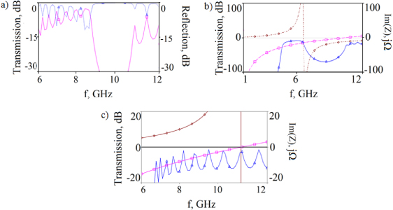
Figure 4. (a) Simulated scattering parameters |S11| (blue, right axis) and |S21| (magenta, left axis) for 20 unit cells. (b) Transmission through 20 unit cells (blue, left axis) and impedance of serial (magenta, right axis) and parallel (blue, right axis) elements for cosφ = 0.2 and fc1 ≠fc2. (c) Transmission through 20 unit cells (blue, left axis) and impedance of serial (magenta, right axis) and parallel (brown, right axis) elements for cosφ = 0.4 and fc1 = fc2.
Download figure:
Standard image High-resolution image3. Experiment
A number of features of the experimental layout have to be restricted to the resolution of the fabrication process of the Josephson junctions. Fortunately, the trilayer process Nb–AlOx–Nb available to us ensures sufficient compactness of the unit cell. This process makes it possible for us to use parallel plate capacitors formed by two niobium layers and an insulation layer from anodic oxide Nb2O5 for all capacitors. Note that the SQUIDs are operating in the superconducting state, and no resistive shunts are used. The layout of the cell, an optical image of the three experimental cells and the wiring at the sample holder are illustrated in figures 5(a)–(c). All six Josephson junctions of each unit cell, which are shown in figure 5(a), are fabricated on a common island. The areas denoted by 5 in figure 5(a) and in dark blue in figure 5(b) are spots where the anodization wiring is etched away at the final stage of the fabrication process. A chip of the size 4 × 4 mm2 contains two completely separated rf transmission lines (i.e. two samples). The two lines are different: one contains 10 and the other contains 20 unit cells per line. The experimental setup is shown in figure 6(a). The samples are measured using an Agilent PNA-X network analyzer in a dry close-cycle cryostat at temperatures about 2 K. Additional attenuators (40 dB) are inserted into the input line in order to reduce the external noise and make sure that the probe rf current does not exceed the critical current of the Josephson junctions. Due to the low probe current, it was necessary to boost the output signal by using a low-noise amplifier (LNA). The magnetic field was applied by a superconducting coil external to the sample holder; the field magnitude is proportional to the current through the coil which is shown in the vertical axis of the following plots.
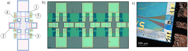
Figure 5. Experimental sample close-up. (a) Cell layout: 1—SQUID loop with large capacitor to ground, 2—via bridge connecting neighboring cells, 3—one of six Josephson junctions of the cell, 4—the bottom electrode is the central island of the cell. (b) Optical microscope image of three cells of the LHTL. (c) Optical microscope image of the connection to the 50-Ω CPW.
Download figure:
Standard image High-resolution image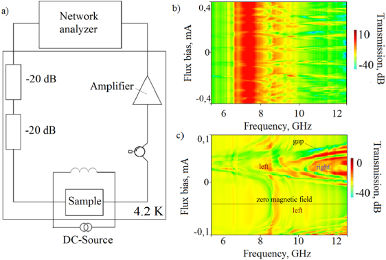
Figure 6. (a) Scheme of the experimental setup. (b) Measured transmission through the transmission line containing 10 cells as function of magnetic field. The magnetic field ranges from −0.4 to 1 mT. No virtual calibration is used. (c) Measured transmission with subtracted background (virtual calibration) for 20-cell line as function of magnetic field. The magnetic field range is between −0.2 and 0.6 mT.
Download figure:
Standard image High-resolution imageMicrowave calibration is not an easy task for cryogenic measurements, as detailed in [13]. Depending on the experimental setup, a proper calibration might not be possible. This is why in this work a virtual calibration for the transmitted signal is attempted. To do this, we averaged the response S21(f,H) for each frequency point, f, over the whole set of data for magnetic field, H, and subtracted the resulting relation  from the measured data. This procedure is feasible since we are interested in detecting the variations caused by the magnetic field at a given frequency, not in frequency variation for a static magnetic field. Since we assume that the relative weight of the large deviation of S caused by H is small, the averaged response
  should deviate slightly from the 'true background'. The transmission through the superconducting LHTL with 10 cells is shown in figure 6(b). No virtual calibration was used here.
One can see from figure 6(b) that the transmission through the line with 10 cells changes periodically with the magnetic field, as expected due to flux quantization. In figure 6(c), we show the transmission with subtracted background  for the line with 20 cells. Here, periodic changes of the transmission with the magnetic field are also observed. At zero field (φ = 0), only one transmission band is seen below 12 GHz. At larger fields cosφ is close enough to zero, and two pass-bands divided by a gap can be seen, as predicted by simulations.
We also observed some discrepancies between simulation and experiment. First, there is moderate transmission below 8 GHz, whereas the simulation predicts negligible transmission (the rejection dip). Second, the frequency range of the rejection band is narrower than predicted. Both these issues can be assigned to a parasitic stray transmission through the sample holder. We simulated this parasitic transmission, which is depicted in figure 7 by the pink curve. The measured rf leak is consistent with the level estimated from the detailed electromagnetic simulations of our sample holder. One can see from figure 7(a) that it is hard to unambiguously extract the cut-off frequency from the experimental data at zero field, not to mention the rejection band limits at relatively large magnetic fields. The unwanted transmission through the holder appears due to, at least, two factors: (i) the holder creates an additional path for the signal, and (ii) the characteristic impedance of the line is strongly mismatched with the 50 Ω input–output lines, as already mentioned. Both these features lead to significant enhancement of the unwanted, but unavoidable rf background and large standing waves in the transmission spectrum as presented in figures 7(a) and (b). To clarify the effect of the rejection gap we subtracted transmission in smaller magnetic field (cosφ = 0.8) from the transmission with larger magnetic field for two cases: (i) with the leaky model of the sample holder (in figure 7(c)) and (ii) with ideal (no-leak) sample holder (in figure 7(d)). From these data one can see that these differential signals are expected to be narrow-band in spite of the fact that the wide-band feature is predicted for an ideal sample holder. The differential signal is predicted to have few dips between the left- and right-handed bands, i.e. between approximately 7 and 11 GHz as presented in figures 7(c) and (d). In this frequency range the transmission is lower in larger magnetic fields than in smaller ones. For both the leaky and the ideal holders the effect is qualitatively the same. This behavior provides a strong indication of the possibility of detecting the predicted gap even with the non-ideal sample holder. The experimental data demonstrate a number of narrow dips as depicted in figure 8. Our virtual calibration via averaging is rather qualitative, so we did not succeed in complete removal of the effect of standing waves in figure 8. Since the impedance of the line changes, the reflected signal (standing wave) also changes with the magnetic field. Nevertheless, the predicted narrow gap is clearly observable: when increasing the magnetic field, it moves to lower frequency and finally disappears, thus merging the left and right-handed bands. Further increase of the magnetic field leads to a reappearance of the gap and makes it deeper again as presented in figure 8. In spite of having observed the rather narrow band gap, this result is supported by the predicted performance as from figures 7(c) and (d).
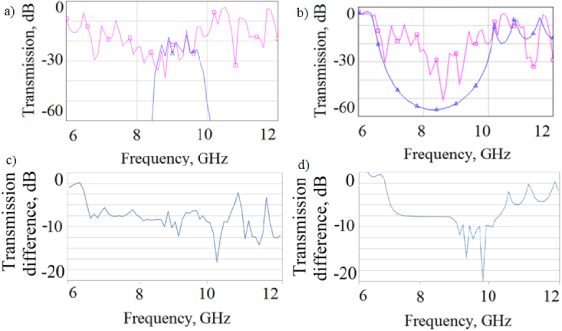
Figure 7. (a) Simulated transmission through the line containing 20 unit cells in the presence of the non-ideal (rf-leaky) sample holder (magenta) and simulation for an ideal (no-leak) sample holder (blue) for a value of cosφ = 0.8. (b) Same data and color coding as in (a), but with cosφ = 0.2. (c) Expected response to magnetic field (from cosφ = 0.2 to 0.8) for the leaky holder as the difference between in transmission (a) and (b). (d) The same difference as in (c) but with an ideal sample holder.
Download figure:
Standard image High-resolution image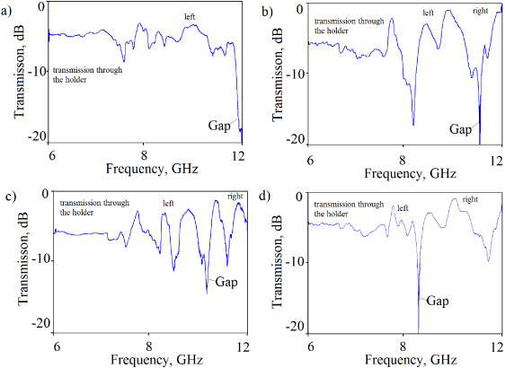
Figure 8. Measured transmission through 20-cell line for various magnetic fields: (a) 0 mT, (b) 0.15 mT, (c) 0.25 mT, and (d) 0.3 mT.
Download figure:
Standard image High-resolution image
4. Conclusion
The concept of a superconducting magnetic field tunable left-handed transmission line with Josephson junctions has passed experimental verification within the frequency range of 6–12 GHz. The calculated dispersion of the line shows left-handed behavior within the lower frequency transmission band. Experimental data demonstrate the tunability of both the transmission and rejection bands by applying a dc magnetic field. The magnetic field allows us to shift the rejection band between the left- and right-handed transmission. Moreover, for a limited frequency range near 10 GHz, the transmission line can be transformed from left-handed to right-handed by changing the magnetic field. The presented experiments are noticeably obscured by parasitic transmission through the sample holder. An improved design of the sample holder is currently under development and we expect to obtain more detailed data in the near future. The potential for improvement may be found in the design of a better impedance match between the sample and the standard 50-Ω cables.
Acknowledgments
This work was supported in part by the Ministry of Education and Science of the Russian Federation, by the Russian Foundation of Basic Research, and by the Deutsche Forschungsgemeinschaft (DFG) and the State of Baden-Württemberg through the DFG Center for Functional Nanostructures (CFN).