


ABSTRACT
The OPAS opacity model has been used to calculate the radiative opacity of stellar plasmas in local thermodynamic equilibrium. According to the recent chemical composition revision of the solar photosphere, opacities have been computed for various hydrogen and metallic element mass fractions. Calculations have been performed toward solar interior modeling for temperatures between ![$\mathrm{log}[T({\rm{K}})]=6$](https://content.cld.iop.org/journals/0067-0049/220/1/2/revision1/apjs518027ieqn1.gif) and
and ![$\mathrm{log}[T({\rm{K}})]=7.2$](https://content.cld.iop.org/journals/0067-0049/220/1/2/revision1/apjs518027ieqn2.gif) , and for electron densities between
, and for electron densities between  and
and  . We discuss possible sources of uncertainty in the calculations. We also compare Rosseland opacities to OPAL and OP data.
Export citation and abstract BibTeX RIS
1. INTRODUCTION
Radiation plays a major role in a wide variety of high energy density astrophysical plasmas. For example, it is well known that the internal temperature profiles of solar-like stars are controlled by the ability of stellar matter to absorb radiation, which can be described in terms of radiative opacity (Eddington 1926). Among the numerous elements making up the stellar chemical composition, metallic elements (elements with atomic number Z greater than two) significantly contribute to the opacity, although they are only present as a few percent of the mixture.
Based on recent refined solar photosphere spectral analysis (Asplund et al. 2009; Scott et al. 2015a, 2015b; Grevesse et al. 2015), the inferred amounts of low-Z metallic elements (mainly carbon, nitrogen, and oxygen) have been revised downward. Standard solar models using such an improved photospheric composition disagree with helioseismic and neutrino observations (Guzik 2008; Serenelli et al. 2009; Turck-Chièze & Couvidat 2011). Among the various proposed explanations, it has been estimated that a smooth increase of the opacity from the range of 2%–5% in the central regions to the range of 12%–15% at the base of the solar convection zone could reconcile models and observations (Serenelli et al. 2009). Such an assumption implies that the opacities of heavier elements in the stellar mixture should be revised upward to compensate for the decreased low-Z metallic element abundances. The focus is on heavier metallic elements because they are always partially ionized in solar-like star interiors. Due to high temperatures, numerous excited atomic states are noticeably populated and significantly contribute to the opacity. Calculations based on an incomplete sampling of such states could lead to opacity values that are too low.
Recently, measurements have been performed of the wavelength-resolved iron opacity at electron temperatures of  and densities of
  (Bailey et al. 2015). These thermodynamic conditions are very similar to those expected near the solar radiation/convection zone boundary. The measured wavelength-resolved opacity appears to be 30%–400% higher than in calculations in a spectral range where L-shell photoexcitation and photoionization processes are prevalent.
Both helioseismic observations and laboratory measurements support the revision of opacity calculations in high energy density plasmas. A large part of the opacity tables commonly used by the astrophysicists community were calculated 20 years ago when computer resources were not what they are today. In order to reduce computational effort, various approximations were made to evaluate the total opacity of the considered mixtures (Iglesias & Rogers 1996; Badnell et al. 2005). Several groups are developing new opacity codes (Porcherot et al. 2011; Blancard et al. 2012; Colgan et al. 2013). Although they differ in their equation of state modeling, all of these codes allow for an extensive detailed line accounting (DLA) based on high-quality atomic structure data obtained in full intermediate coupling. The OPAS opacity model has recently been used to calculate the solar opacities along a specific thermodynamical path (Blancard et al. 2012). In the present work, we used this model to produce opacity tables that are useful for solar radiative zone modeling. According to the AGS'09 composition (Asplund et al. 2009), a mixture including the 22 most abundant chemical elements has been considered (abundance greater or almost equal to 5). Hence, cobalt has been added to the 21 element list considered in OPAL calculations (Iglesias & Rogers 1996). Possible sources of uncertainty in the calculations are examined and discussed. The Rosseland opacities that we obtained are compared to OP (http://cdsweb.u-strasbg.fr/topbase/topbase.html) and OPAL (http://opalopacity.llnl.gov) data.
2. NUMERICAL PROCEDURES
The OPAS opacity code has been described previously (Blancard et al. 2012). We simply note that it has been developed in the detailed configuration accounting framework. The monochromatic opacity is evaluated as a sum of four contributions involving the diffusion process as free–free, bound–free, and bound–bound absorption processes. The bound–bound opacity is calculated by combining various approximations to take into account the level structure of configurations. In any case, statistical methods are used to describe the electric-dipole transition arrays connecting two non-relativistic configurations. When necessary, and computationally manageable, the statistical description of the transition arrays is replaced by an extensive DLA performed in the full intermediate coupling scheme from jj-coupling. For stellar opacity tabulations, such an approach is the best compromise between accuracy and computational time.
Since its first use to calculate solar opacities, the OPAS code has been improved by including a systematic ionic Stark broadening treatment. In hot dense plasmas, highly excited atomic states can be notably populated. Photoexcitation processes from these atomic states give rise to satellite lines that can significantly overlap and merge with resonance lines due to broadening mechanisms acting on the overall lines. The Stark effect can be an important source of line broadening. For hot dense plasmas, it results from the existence of fluctuating electric fields produced by both free electrons and slow-moving ions. Splitting levels into sublevels, these electric fields can significantly modify the atomic bound states, together with the wavelengths and strengths of the transitions connecting these states. The perturbing field induced by the ions is described here using the quasi-static approximation. The electric microfield distribution we considered depends on the considered mixture. It is evaluated as a sum over the chemical elements of the individual electric microfield distributions weighted by the element number fraction in the mixture. For hydrogen-like and helium-like ions, the initial line broadening treatment has been retained. We note that it is based on the standard theory including linear the Stark theory (Griem 1997). For a given electric microfield distribution, spectral line profiles are computed following methods developed by Lee (1988). For the other ionic stages, statistical ionic Stark broadening is applied using a model proposed by Rozsnyai (1977).
Opacity calculations dedicated to the solar interior have been performed for temperatures between ![$\mathrm{log}[T({\rm{K}})]=6$](https://content.cld.iop.org/journals/0067-0049/220/1/2/revision1/apjs518027ieqn7.gif) and
and ![$\mathrm{log}[T({\rm{K}})]=7.2$](https://content.cld.iop.org/journals/0067-0049/220/1/2/revision1/apjs518027ieqn8.gif) . The electron density has been sampled between
. The electron density has been sampled between ![$\mathrm{log}[{N}_{{\rm{e}}}({\mathrm{cm}}^{-3})]=20$](https://content.cld.iop.org/journals/0067-0049/220/1/2/revision1/apjs518027ieqn9.gif) and
and ![$\mathrm{log}[{N}_{{\rm{e}}}({\mathrm{cm}}^{-3})]=26$](https://content.cld.iop.org/journals/0067-0049/220/1/2/revision1/apjs518027ieqn10.gif) . An iso-thermal iso-Ne mixing model is used to evaluate the opacity of the mixture. For a given Ne value, the partial density of each element in the mixture is determined. The density of the mixture (ρ) is deduced from the additivity of the partial volumes. The opacity of the mixture is expressed as a weighted sum of individual opacities computed at the partial density of interest. The refined electron density sampling we used allows for an accurate interpolation of our Rosseland opacity values on a
. An iso-thermal iso-Ne mixing model is used to evaluate the opacity of the mixture. For a given Ne value, the partial density of each element in the mixture is determined. The density of the mixture (ρ) is deduced from the additivity of the partial volumes. The opacity of the mixture is expressed as a weighted sum of individual opacities computed at the partial density of interest. The refined electron density sampling we used allows for an accurate interpolation of our Rosseland opacity values on a ![$\mathrm{log}[R]$](https://content.cld.iop.org/journals/0067-0049/220/1/2/revision1/apjs518027ieqn11.gif) -grid (where
-grid (where  , with
  and ρ expressed in
  ).
).
3. UNCERTAINTY EVALUATION
3.1. Equation of State
Because they are prevalent at solar interior temperatures, an exhaustive and accurate description of excited atomic states is crucial to correctly evaluate opacities. In stellar interiors, the number and energy of these atomic states strongly depend on the approach employed to describe the plasma environment effects.
In order to illustrate this point, we focused on iron opacity. Three thermodynamical conditions are considered, ![$\{\mathrm{log}[T({\rm{K}})],\mathrm{log}[{N}_{{\rm{e}}}({\mathrm{cm}}^{-3})])\}$](https://content.cld.iop.org/journals/0067-0049/220/1/2/revision1/apjs518027ieqn15.gif) =
=  ,
,  , and
, and  , for which iron is a major metallic contributor to the mixture opacity (Figure 1). Concerning the Sun, these thermodynamical conditions are similar to those expected near the radiation/convection boundary, the middle of the radiative zone, and the center, respectively. For each case, the OPAS configuration probabilities are replaced by those obtained by solving Saha–Boltzmann equations and using the configuration energies of isolated ions corrected by plasma environment effects. These effects are deduced from either an ion sphere (IS) model (Massacrier & Dubau 1990) or the Stewart–Pyatt (SP) model (Stewart & Pyatt 1966). The isolated ion configuration energies are simply evaluated using a screened hydrogenic model including ℓ-splitting (Faussurier et al. 1997). The average ionization, the lowest bound subshell, the number of retained non-relativistic configurations, and the iron Rosseland opacity are given in Table 1, which also contains the OPAS values. IS and OPAS average ionizations are close to whatever thermodynamical conditions we considered. Except for the (
![$\mathrm{log}[T({\rm{K}})]=7.20$](https://content.cld.iop.org/journals/0067-0049/220/1/2/revision1/apjs518027ieqn19.gif) ,
, ![$\mathrm{log}[{N}_{{\rm{e}}}({\mathrm{cm}}^{-3})]=25.8$](https://content.cld.iop.org/journals/0067-0049/220/1/2/revision1/apjs518027ieqn20.gif) ) case, IS ionization standard deviations are lower than the OPAS values, leading to a lower iron Rosseland opacity. Compared to the OPAS values, the SP average ionizations are systematically lower because the plasma environment effect modeling induces smaller configuration energy corrections. Depending on the thermodynamical conditions, the ratios of IS and SP iron Rosseland opacities to the OPAS values equal
) case, IS ionization standard deviations are lower than the OPAS values, leading to a lower iron Rosseland opacity. Compared to the OPAS values, the SP average ionizations are systematically lower because the plasma environment effect modeling induces smaller configuration energy corrections. Depending on the thermodynamical conditions, the ratios of IS and SP iron Rosseland opacities to the OPAS values equal  and
and  , respectively. Mixture Rosseland opacities have been calculated by replacing the OPAS iron spectral opacity by the IS and SP calculations for
  The
The  ratio equals
  ,
,  , and
, and  for the three thermodynamical conditions we considered.

Figure 1. Relative contributions of each element to the OPAS Rosseland opacities (AGS'09 composition,  ) for
) for ![$\{\mathrm{log}[T({\rm{K}})],\mathrm{log}[{N}_{{\rm{e}}}({\mathrm{cm}}^{-3})]\}$](https://content.cld.iop.org/journals/0067-0049/220/1/2/revision1/apjs518027ieqn29.gif) =
=  (upper panel),
  (middle panel), and
  (lower panel). Scattering (gray), free–free (black), bound–free (blue), and bound–bound (red) contributions are indicated.
Download figure:
Standard image High-resolution imageTable 1. Equation of State of Iron and its Influence on the Rosseland Mean Opacities for Typical Solar Conditions
| Z* |

|
nℓmax | Conf |

|

|
|
| 16.29 | 1.255 | 6s | 44746 | 1350.9 | 24.88 | |
| A | 16.43 | 1.196 | 6h | 23607 | 1196.4 | 24.64 |
| 15.29 | 1.375 | 8k | 60661 | 1576.6 | 25.34 | |
| 20.17 | 1.418 | 3d | 1092 | 290.8 | 4.53 | |
| B | 20.14 | 1.181 | 4f | 890 | 264.5 | 4.47 |
| 19.06 | 1.586 | 5g | 6836 | 309.6 | 4.57 | |
| 22.08 | 1.173 | 2p | 59 | 120.3 | 1.38 | |
| C | 21.98 | 1.186 | 2p | 51 | 121.3 | 1.39 |
| 21.05 | 0.882 | 3d | 369 | 106.9 | 1.37 |
Note. OPAS, IS (Ionic Sphere), and SP (Stewart Pyatt) values are given on the upper, mid, and lower lines, respectively. Opacity is expressed in  .
.
Average Ionization (Z*), Ionization Standard Deviation ( ), Lowest Bound Subshell (nℓmax), Number of Selected Non-relativistic Configurations (Conf), Iron Rosseland Opacity (
 ), and 22 Chemical Element Mixture (AGS'09 Composition,
  ) Rosseland Opacity (
 ) for
) for ![$\{\mathrm{log}[T({\rm{K}})],\mathrm{log}[{N}_{{\rm{e}}}({\mathrm{cm}}^{-3})]\}$](https://content.cld.iop.org/journals/0067-0049/220/1/2/revision1/apjs518027ieqn37.gif) =
=  (A),
(A),  (B), and
  (C)
(C)
Download table as: ASCIITypeset image
We also examined the impact of excited configuration sampling. Based on the IS model, Saha–Boltzmann equations have been solved considering, for each ionic state, multiple excitations from the ground configuration valence shell. The results in Table 1 have been obtained considering up to triple excitations. Downgraded calculations have also been performed where the excited configuration sampling has been restricted to single and double excitations. The resulting iron spectral opacities for ![$\mathrm{log}[T({\rm{K}})]=6.35$](https://content.cld.iop.org/journals/0067-0049/220/1/2/revision1/apjs518027ieqn45.gif) and
and ![$\mathrm{log}[{N}_{{\rm{e}}}({\mathrm{cm}}^{-3})]=23$](https://content.cld.iop.org/journals/0067-0049/220/1/2/revision1/apjs518027ieqn46.gif) are plotted in Figure 2. The contribution of M-shell bound–free absorption from excited configurations is clearly visible near u = 3 (u is the reduced photon energy defined as
are plotted in Figure 2. The contribution of M-shell bound–free absorption from excited configurations is clearly visible near u = 3 (u is the reduced photon energy defined as  , where h, ν, and
  are the Planck constant, the frequency, and the Boltzmann constant, respectively). The iron Rosseland opacities equal 906.0 and
  for single and double excitations, respectively. Using these iron spectral opacities, mixture Rosseland opacities (
 ) equal 24.603 and 24.641 for single and double excitations, which are very close to the nominal IS calculation (24.642).
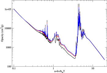
Figure 2. Iron opacities for ![$\mathrm{log}[T({\rm{K}})]=6.35$](https://content.cld.iop.org/journals/0067-0049/220/1/2/revision1/apjs518027ieqn51.gif) and
and ![$\mathrm{log}[{N}_{{\rm{e}}}({\mathrm{cm}}^{-3})]=23$](https://content.cld.iop.org/journals/0067-0049/220/1/2/revision1/apjs518027ieqn52.gif) . Single (black curve), double (red curve), and triple (blue curve) excitations from the valence shell of the ground configuration of each ionic state are considered.
. Single (black curve), double (red curve), and triple (blue curve) excitations from the valence shell of the ground configuration of each ionic state are considered.
Download figure:
Standard image High-resolution imageThe evaluation of excited configuration energies can be another source of uncertainty. We recall that OPAS uses the notion of superconfiguration characterized by a set a supershells where each of them can be defined by one or several sub-shells up to several spectroscopic shells. For each superconfiguration, a set of one-electron radial wavefunctions is optimized while minimizing the statistical average of the energy levels that the superconfiguration contains. Forcing each spectroscopic shell to be a supershell, we increase the number of initially generated superconfigurations by approximately one order of magnitude, improving the energy calculation accuracy of the configurations contained in a given superconfiguration. Concerning the iron opacity for ![$\mathrm{log}[T({\rm{K}})]=6.35$](https://content.cld.iop.org/journals/0067-0049/220/1/2/revision1/apjs518027ieqn53.gif) and
and ![$\mathrm{log}[{N}_{{\rm{e}}}({\mathrm{cm}}^{-3})]=23$](https://content.cld.iop.org/journals/0067-0049/220/1/2/revision1/apjs518027ieqn54.gif) , we found that
, we found that  has decreased by
  . Concerning the stellar mixture for the same thermodynamical conditions, the Rosseland opacity decrease is less than
  for (
for ( ).
).
3.2. Detailed Line Accounting
The OPAS bound–bound opacity calculation combines statistical (Unresolved Transition Array; UTA) and DLA descriptions of electric-dipole transition arrays. We note that opacities are calculated in the ![$[0.1,20]$](https://content.cld.iop.org/journals/0067-0049/220/1/2/revision1/apjs518027ieqn59.gif) reduced photon energy range. For each transition array connecting two non-relativistic configurations, the DLA is applied for
reduced photon energy range. For each transition array connecting two non-relativistic configurations, the DLA is applied for ![$u\in [0.2,13.5]$](https://content.cld.iop.org/journals/0067-0049/220/1/2/revision1/apjs518027ieqn60.gif) only if the number of lines is smaller than 106 and if the line overlap criteria, defined as the ratio of the average Doppler width to the average energy separation between two lines, is lower than 10. These values have been retained to ensure an exhaustive DLA treatment.
only if the number of lines is smaller than 106 and if the line overlap criteria, defined as the ratio of the average Doppler width to the average energy separation between two lines, is lower than 10. These values have been retained to ensure an exhaustive DLA treatment.
In order to examine the impact of a DLA treatment, the mixture opacity calculations have been performed while forcing a statistical treatment for the overall transition arrays. The results obtained using this downgraded OPAS version (dOPAS) have been compared to standard OPAS calculations. Figure 3 shows the relative variation  for (
for ( ). If ratio values are always positive in the considered thermodynamical domain, then the impact of the DLA treatment remains moderate. The larger differences can be observed in the range of low
 ![$\mathrm{log}[T]$](https://content.cld.iop.org/journals/0067-0049/220/1/2/revision1/apjs518027ieqn63.gif) and low
and low ![$\mathrm{log}[R]$](https://content.cld.iop.org/journals/0067-0049/220/1/2/revision1/apjs518027ieqn64.gif) values. The largest difference is
values. The largest difference is  for
for ![$\mathrm{log}[T({\rm{K}})]=6.0$](https://content.cld.iop.org/journals/0067-0049/220/1/2/revision1/apjs518027ieqn66.gif) ,
, ![$\mathrm{log}[R]=-2.0$](https://content.cld.iop.org/journals/0067-0049/220/1/2/revision1/apjs518027ieqn67.gif) . At low temperatures, the Doppler width involved in the line overlap criteria is small enough to allow a DLA treatment both for the K-shell of low-Z elements and for the L-shell of the heavier elements for which a lot of UTA contain a large number of lines. At a fixed temperature, the spectral distribution of a given resolved transition array is smoothed when the density increases. Electron collision broadening is an efficient broadening process that acts on each line of the transition array. Such a process mainly contributes to fill the spectral gap between lines. The opacity of the stellar mixture results from the accumulation of such smoothed spectral distributions showing an absorption background not much different from that obtained using the systematic statistical treatment for the overall transition arrays. Remembering that the Rosseland opacity is a harmonic average of the monochromatic opacity, the
. At low temperatures, the Doppler width involved in the line overlap criteria is small enough to allow a DLA treatment both for the K-shell of low-Z elements and for the L-shell of the heavier elements for which a lot of UTA contain a large number of lines. At a fixed temperature, the spectral distribution of a given resolved transition array is smoothed when the density increases. Electron collision broadening is an efficient broadening process that acts on each line of the transition array. Such a process mainly contributes to fill the spectral gap between lines. The opacity of the stellar mixture results from the accumulation of such smoothed spectral distributions showing an absorption background not much different from that obtained using the systematic statistical treatment for the overall transition arrays. Remembering that the Rosseland opacity is a harmonic average of the monochromatic opacity, the  values deduced from standard and downgraded OPAS calculations are quite similar when the density increases. Our results confirm those previously obtained for highly diluted and low-temperature astrophysical plasmas (Iglesias & Wilson 1994).
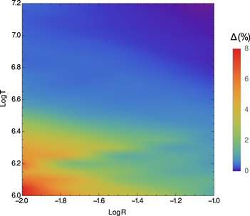
Figure 3. Comparison of OPAS Rosseland opacities ( ) for a 22 elements solar mixture at (AGS'09 composition,
  ) with DLA treatment (OPAS) or without it (dOPAS).
Download figure:
Standard image High-resolution image3.3. Electric Microfield Distribution and Ionic Stark Broadening Modeling
In order to estimate the sensitivity of the opacities with the electric microfields, in Figure 4 we compare the nominal  OPAS values for (
 ) and the results deduced from downgraded computations where spectra are computed using the (
 ) microfield distribution and mixed according to the (
 ) composition. The difference between the two calculations appears to be quite small and always lower than or equal to zero. The largest discrepancy (
 ) is found for (
![$\mathrm{log}[R]=-1.95$](https://content.cld.iop.org/journals/0067-0049/220/1/2/revision1/apjs518027ieqn76.gif) ,
, ![$\mathrm{log}[T({\rm{K}})]=6.15)$](https://content.cld.iop.org/journals/0067-0049/220/1/2/revision1/apjs518027ieqn77.gif) . For these thermodynamical conditions, the average electric field values equal 0.112 and 0.100 atomic units for (
. For these thermodynamical conditions, the average electric field values equal 0.112 and 0.100 atomic units for ( ) and (
 ), respectively. These average values are used to evaluate the statistical ionic Stark broadening applied (except for H-like and He-like ions for which a refined treatment is used) to the overall transition arrays. If the mixture Rosseland opacities weakly depend on the electric microfield distribution modeling, then we find that the statistical ionic Stark broadening treatment recently implemented in the OPAS code noticeably increases their values for low-density and low-temperature plasmas. For such media, photoexcitation processes from partially ionized metallic elements significantly contribute to the total opacity (see upper panel on Figure 1). As an example, the ratio of the 22 chemical element mixture Rosseland opacity calculated with and without statistical ionic Stark broadening for (
![$\mathrm{log}[T({\rm{K}})]=6.35$](https://content.cld.iop.org/journals/0067-0049/220/1/2/revision1/apjs518027ieqn80.gif) ,
, ![$\mathrm{log}[{N}_{{\rm{e}}}({\mathrm{cm}}^{-3})]=23$](https://content.cld.iop.org/journals/0067-0049/220/1/2/revision1/apjs518027ieqn81.gif) ) and (
) and ( ) equals 1.015. The validity of our statistical ionic Stark broadening treatment remains a source of uncertainty that could be quantified by performing systematic detailed Stark broadening calculations. Unfortunately, such calculations are presently impracticable for complex N-electron atomic structures.

Figure 4. Comparison of OPAS Rosseland opacities ( ) for a 22 element solar mixture at
  using microfields from (
 ) or (
 ). The AGS'09 composition is used for both.
Download figure:
Standard image High-resolution image3.4. Interpolation
Because our Rosseland opacity computations are performed on a ![$\mathrm{log}[{N}_{{\rm{e}}}]$](https://content.cld.iop.org/journals/0067-0049/220/1/2/revision1/apjs518027ieqn87.gif) -grid, an interpolation is necessary to obtain the projected values on a standard
-grid, an interpolation is necessary to obtain the projected values on a standard ![$\mathrm{log}[R]$](https://content.cld.iop.org/journals/0067-0049/220/1/2/revision1/apjs518027ieqn88.gif) -grid. This process contributes to the uncertainty and needs to be detailed. For each T value, a cubic spline as a function of
-grid. This process contributes to the uncertainty and needs to be detailed. For each T value, a cubic spline as a function of ![$\mathrm{log}[R]$](https://content.cld.iop.org/journals/0067-0049/220/1/2/revision1/apjs518027ieqn89.gif) is optimized by choosing the free parameters couple that minimizes the standard deviation of the interpolation errors. Concretely, we compute an interpolation error on a spline node as the relative difference between the actual value and that obtained through the spline that does not take this node into account. Depending on the temperature, up to
is optimized by choosing the free parameters couple that minimizes the standard deviation of the interpolation errors. Concretely, we compute an interpolation error on a spline node as the relative difference between the actual value and that obtained through the spline that does not take this node into account. Depending on the temperature, up to  can be reached by a residual standard deviation and 1% by an extreme individual interpolation error. These errors could be reduced by a finer
 ![$\mathrm{log}[{N}_{{\rm{e}}}]$](https://content.cld.iop.org/journals/0067-0049/220/1/2/revision1/apjs518027ieqn91.gif) sampling, but it should be noted that they are already of the same magnitude as the other uncertainty sources. Moreover, OPAS tables are given on a fine
sampling, but it should be noted that they are already of the same magnitude as the other uncertainty sources. Moreover, OPAS tables are given on a fine ![$\mathrm{log}[R]$](https://content.cld.iop.org/journals/0067-0049/220/1/2/revision1/apjs518027ieqn92.gif) -mesh with the goal of minimizing further errors due to external interpolation procedures. We note that, contrary to OPAL tables, no smoothing filter is applied to our data before interpolation.
-mesh with the goal of minimizing further errors due to external interpolation procedures. We note that, contrary to OPAL tables, no smoothing filter is applied to our data before interpolation.
4. OPAS ROSSELAND OPACITY TABULATIONS
OPAS Rosseland opacities have been tabulated for ![$\mathrm{log}[R]$](https://content.cld.iop.org/journals/0067-0049/220/1/2/revision1/apjs518027ieqn93.gif) in the range
in the range ![$[-2,-1]$](https://content.cld.iop.org/journals/0067-0049/220/1/2/revision1/apjs518027ieqn94.gif) (step = 0.05) and for
(step = 0.05) and for ![$\mathrm{log}[T({\rm{K}})]$](https://content.cld.iop.org/journals/0067-0049/220/1/2/revision1/apjs518027ieqn95.gif) in the range
in the range ![$[6,7.2]$](https://content.cld.iop.org/journals/0067-0049/220/1/2/revision1/apjs518027ieqn96.gif) (step = 0.025). Hydrogen mass fractions equaling
(step = 0.025). Hydrogen mass fractions equaling  , 0.2, 0.35, 0.5, 0.7, and 0.8 have been considered. For each X value, metallic element mass fractions equal to 0.01, 0.013, 0.015, 0.017, and 0.02 have been retained. Table 2 illustrates the available data for
  . We note that for the overall considered thermodynamical conditions, the cobalt contribution to the mixture Rosseland opacity is negligible. Greater relative Co contributions are found for higher temperatures but are always lower than
  .
.
Table 2.
![$\mathrm{log}[{\kappa }_{{\rm{R}}}({\mathrm{cm}}^{2}\;{{\rm{g}}}^{-1})]$](https://content.cld.iop.org/journals/0067-0049/220/1/2/revision1/apjs518027ieqn100.gif) for AGS'09 Composition and Mass Fractions X = 0.350 and Z = 0.020
for AGS'09 Composition and Mass Fractions X = 0.350 and Z = 0.020
| −2.000 | −1.950 | −1.900 | −1.850 | −1.800 | −1.750 | −1.700 | −1.650 | −1.600 | −1.550 | −1.500 | −1.450 | −1.400 | −1.350 | −1.300 | -1.250 | −1.200 | −1.150 | −1.100 | −1.050 | −1.000 | |
|---|---|---|---|---|---|---|---|---|---|---|---|---|---|---|---|---|---|---|---|---|---|
| 6.000 | 1.463 | 1.498 | 1.533 | 1.567 | 1.600 | 1.633 | 1.664 | 1.695 | 1.724 | 1.752 | 1.779 | 1.806 | 1.834 | 1.863 | 1.893 | 1.923 | 1.951 | 1.977 | 2.000 | 2.021 | 2.041 |
| 6.025 | 1.432 | 1.468 | 1.505 | 1.540 | 1.574 | 1.607 | 1.638 | 1.667 | 1.695 | 1.724 | 1.755 | 1.788 | 1.821 | 1.852 | 1.881 | 1.905 | 1.928 | 1.949 | 1.971 | 1.995 | 2.019 |
| 6.050 | 1.404 | 1.441 | 1.477 | 1.512 | 1.547 | 1.580 | 1.611 | 1.643 | 1.674 | 1.706 | 1.739 | 1.773 | 1.805 | 1.834 | 1.860 | 1.883 | 1.905 | 1.927 | 1.950 | 1.974 | 2.000 |
| 6.075 | 1.379 | 1.416 | 1.452 | 1.487 | 1.521 | 1.555 | 1.588 | 1.623 | 1.657 | 1.692 | 1.726 | 1.757 | 1.786 | 1.812 | 1.837 | 1.860 | 1.884 | 1.908 | 1.932 | 1.957 | 1.982 |
| 6.100 | 1.356 | 1.394 | 1.430 | 1.465 | 1.500 | 1.535 | 1.571 | 1.607 | 1.643 | 1.678 | 1.710 | 1.739 | 1.765 | 1.790 | 1.814 | 1.839 | 1.865 | 1.891 | 1.917 | 1.942 | 1.966 |
| 6.125 | 1.336 | 1.374 | 1.412 | 1.449 | 1.486 | 1.523 | 1.559 | 1.595 | 1.629 | 1.661 | 1.690 | 1.717 | 1.743 | 1.769 | 1.795 | 1.822 | 1.849 | 1.876 | 1.902 | 1.927 | 1.951 |
| 6.150 | 1.318 | 1.358 | 1.397 | 1.436 | 1.475 | 1.512 | 1.548 | 1.582 | 1.612 | 1.641 | 1.668 | 1.695 | 1.722 | 1.751 | 1.779 | 1.807 | 1.834 | 1.860 | 1.886 | 1.911 | 1.935 |
| 6.175 | 1.304 | 1.345 | 1.386 | 1.426 | 1.464 | 1.499 | 1.532 | 1.562 | 1.591 | 1.619 | 1.647 | 1.676 | 1.705 | 1.734 | 1.762 | 1.790 | 1.817 | 1.843 | 1.868 | 1.892 | 1.915 |
| 6.200 | 1.293 | 1.335 | 1.375 | 1.413 | 1.449 | 1.481 | 1.511 | 1.540 | 1.569 | 1.599 | 1.629 | 1.659 | 1.688 | 1.717 | 1.744 | 1.771 | 1.797 | 1.822 | 1.846 | 1.869 | 1.892 |
| 6.225 | 1.285 | 1.323 | 1.360 | 1.394 | 1.427 | 1.458 | 1.488 | 1.518 | 1.549 | 1.580 | 1.611 | 1.641 | 1.670 | 1.697 | 1.723 | 1.748 | 1.773 | 1.797 | 1.820 | 1.842 | 1.864 |
| 6.250 | 1.274 | 1.309 | 1.341 | 1.372 | 1.403 | 1.434 | 1.465 | 1.497 | 1.529 | 1.561 | 1.591 | 1.620 | 1.647 | 1.674 | 1.699 | 1.723 | 1.746 | 1.768 | 1.790 | 1.811 | 1.832 |
| 6.275 | 1.256 | 1.289 | 1.320 | 1.351 | 1.382 | 1.413 | 1.445 | 1.476 | 1.507 | 1.536 | 1.565 | 1.593 | 1.620 | 1.645 | 1.670 | 1.694 | 1.716 | 1.737 | 1.758 | 1.777 | 1.796 |
| 6.300 | 1.234 | 1.266 | 1.298 | 1.330 | 1.361 | 1.393 | 1.423 | 1.453 | 1.481 | 1.509 | 1.536 | 1.562 | 1.588 | 1.612 | 1.636 | 1.659 | 1.680 | 1.701 | 1.721 | 1.739 | 1.757 |
| 6.325 | 1.212 | 1.244 | 1.277 | 1.308 | 1.339 | 1.369 | 1.398 | 1.425 | 1.452 | 1.479 | 1.504 | 1.529 | 1.552 | 1.575 | 1.596 | 1.617 | 1.638 | 1.658 | 1.678 | 1.696 | 1.714 |
| 6.350 | 1.190 | 1.222 | 1.254 | 1.285 | 1.314 | 1.341 | 1.368 | 1.394 | 1.420 | 1.445 | 1.470 | 1.493 | 1.514 | 1.534 | 1.553 | 1.572 | 1.592 | 1.611 | 1.631 | 1.650 | 1.668 |
| 6.375 | 1.167 | 1.198 | 1.228 | 1.256 | 1.283 | 1.310 | 1.335 | 1.360 | 1.384 | 1.408 | 1.431 | 1.452 | 1.472 | 1.490 | 1.508 | 1.526 | 1.544 | 1.563 | 1.582 | 1.600 | 1.618 |
| 6.400 | 1.140 | 1.169 | 1.196 | 1.223 | 1.248 | 1.274 | 1.298 | 1.322 | 1.345 | 1.366 | 1.387 | 1.407 | 1.426 | 1.444 | 1.462 | 1.479 | 1.496 | 1.513 | 1.531 | 1.548 | 1.565 |
| 6.425 | 1.106 | 1.133 | 1.159 | 1.185 | 1.209 | 1.233 | 1.256 | 1.279 | 1.300 | 1.321 | 1.341 | 1.360 | 1.378 | 1.395 | 1.412 | 1.429 | 1.445 | 1.462 | 1.478 | 1.494 | 1.510 |
| 6.450 | 1.067 | 1.093 | 1.118 | 1.143 | 1.166 | 1.189 | 1.211 | 1.232 | 1.253 | 1.272 | 1.291 | 1.310 | 1.327 | 1.345 | 1.361 | 1.377 | 1.393 | 1.408 | 1.424 | 1.439 | 1.454 |
| 6.475 | 1.026 | 1.050 | 1.074 | 1.097 | 1.120 | 1.142 | 1.163 | 1.184 | 1.203 | 1.222 | 1.240 | 1.258 | 1.276 | 1.293 | 1.309 | 1.325 | 1.339 | 1.353 | 1.368 | 1.383 | 1.398 |
| 6.500 | 0.982 | 1.004 | 1.027 | 1.050 | 1.072 | 1.093 | 1.114 | 1.134 | 1.152 | 1.170 | 1.188 | 1.206 | 1.223 | 1.240 | 1.256 | 1.270 | 1.284 | 1.298 | 1.312 | 1.327 | 1.344 |
| 6.525 | 0.935 | 0.957 | 0.978 | 1.000 | 1.021 | 1.042 | 1.063 | 1.082 | 1.101 | 1.118 | 1.136 | 1.152 | 1.169 | 1.184 | 1.199 | 1.213 | 1.228 | 1.242 | 1.257 | 1.273 | 1.290 |
| 6.550 | 0.886 | 0.907 | 0.928 | 0.948 | 0.969 | 0.989 | 1.009 | 1.029 | 1.047 | 1.065 | 1.082 | 1.098 | 1.113 | 1.127 | 1.142 | 1.157 | 1.172 | 1.188 | 1.204 | 1.221 | 1.237 |
| 6.575 | 0.835 | 0.856 | 0.876 | 0.896 | 0.916 | 0.936 | 0.955 | 0.973 | 0.992 | 1.009 | 1.026 | 1.041 | 1.057 | 1.072 | 1.087 | 1.103 | 1.119 | 1.135 | 1.152 | 1.168 | 1.185 |
| 6.600 | 0.784 | 0.805 | 0.825 | 0.844 | 0.863 | 0.881 | 0.899 | 0.917 | 0.934 | 0.951 | 0.968 | 0.985 | 1.001 | 1.018 | 1.034 | 1.050 | 1.066 | 1.083 | 1.099 | 1.115 | 1.132 |
| 6.625 | 0.732 | 0.753 | 0.772 | 0.791 | 0.809 | 0.826 | 0.843 | 0.861 | 0.878 | 0.895 | 0.912 | 0.929 | 0.946 | 0.963 | 0.980 | 0.996 | 1.012 | 1.028 | 1.045 | 1.061 | 1.078 |
| 6.650 | 0.678 | 0.699 | 0.718 | 0.736 | 0.753 | 0.770 | 0.787 | 0.804 | 0.821 | 0.839 | 0.856 | 0.874 | 0.891 | 0.909 | 0.925 | 0.942 | 0.958 | 0.974 | 0.990 | 1.007 | 1.025 |
| 6.675 | 0.621 | 0.641 | 0.660 | 0.678 | 0.696 | 0.713 | 0.731 | 0.748 | 0.766 | 0.783 | 0.801 | 0.819 | 0.836 | 0.853 | 0.870 | 0.887 | 0.904 | 0.921 | 0.938 | 0.956 | 0.974 |
| 6.700 | 0.563 | 0.582 | 0.601 | 0.620 | 0.638 | 0.657 | 0.675 | 0.693 | 0.711 | 0.728 | 0.746 | 0.763 | 0.780 | 0.798 | 0.815 | 0.833 | 0.851 | 0.869 | 0.887 | 0.905 | 0.922 |
| 6.725 | 0.506 | 0.524 | 0.543 | 0.562 | 0.582 | 0.601 | 0.620 | 0.639 | 0.657 | 0.674 | 0.691 | 0.708 | 0.726 | 0.744 | 0.763 | 0.782 | 0.800 | 0.818 | 0.835 | 0.852 | 0.870 |
| 6.750 | 0.450 | 0.469 | 0.488 | 0.507 | 0.527 | 0.547 | 0.566 | 0.585 | 0.603 | 0.620 | 0.637 | 0.655 | 0.673 | 0.692 | 0.712 | 0.731 | 0.749 | 0.766 | 0.783 | 0.801 | 0.819 |
| 6.775 | 0.397 | 0.416 | 0.435 | 0.454 | 0.474 | 0.493 | 0.512 | 0.531 | 0.549 | 0.567 | 0.585 | 0.604 | 0.623 | 0.642 | 0.661 | 0.679 | 0.697 | 0.715 | 0.734 | 0.753 | 0.772 |
| 6.800 | 0.345 | 0.365 | 0.385 | 0.404 | 0.422 | 0.441 | 0.459 | 0.478 | 0.497 | 0.516 | 0.536 | 0.555 | 0.575 | 0.593 | 0.611 | 0.629 | 0.648 | 0.667 | 0.687 | 0.707 | 0.728 |
| 6.825 | 0.296 | 0.315 | 0.335 | 0.353 | 0.372 | 0.390 | 0.409 | 0.429 | 0.449 | 0.469 | 0.488 | 0.508 | 0.526 | 0.545 | 0.563 | 0.583 | 0.602 | 0.623 | 0.643 | 0.664 | 0.685 |
| 6.850 | 0.248 | 0.267 | 0.286 | 0.305 | 0.324 | 0.343 | 0.363 | 0.383 | 0.404 | 0.423 | 0.443 | 0.461 | 0.480 | 0.499 | 0.519 | 0.540 | 0.561 | 0.581 | 0.602 | 0.623 | 0.643 |
| 6.875 | 0.203 | 0.221 | 0.240 | 0.259 | 0.279 | 0.300 | 0.320 | 0.340 | 0.360 | 0.379 | 0.398 | 0.418 | 0.438 | 0.458 | 0.479 | 0.500 | 0.521 | 0.542 | 0.563 | 0.584 | 0.606 |
| 6.900 | 0.160 | 0.179 | 0.199 | 0.219 | 0.239 | 0.260 | 0.280 | 0.300 | 0.319 | 0.338 | 0.358 | 0.379 | 0.400 | 0.421 | 0.443 | 0.464 | 0.485 | 0.506 | 0.527 | 0.550 | 0.573 |
| 6.925 | 0.122 | 0.142 | 0.162 | 0.183 | 0.203 | 0.223 | 0.242 | 0.261 | 0.281 | 0.302 | 0.323 | 0.345 | 0.366 | 0.388 | 0.410 | 0.431 | 0.452 | 0.474 | 0.497 | 0.520 | 0.544 |
| 6.950 | 0.089 | 0.109 | 0.130 | 0.150 | 0.169 | 0.188 | 0.208 | 0.227 | 0.248 | 0.270 | 0.292 | 0.314 | 0.336 | 0.358 | 0.379 | 0.401 | 0.424 | 0.447 | 0.470 | 0.494 | 0.519 |
| 6.975 | 0.060 | 0.080 | 0.099 | 0.119 | 0.139 | 0.158 | 0.179 | 0.200 | 0.222 | 0.243 | 0.265 | 0.287 | 0.309 | 0.331 | 0.353 | 0.376 | 0.399 | 0.423 | 0.447 | 0.471 | 0.496 |
| 7.000 | 0.035 | 0.053 | 0.072 | 0.092 | 0.112 | 0.133 | 0.155 | 0.177 | 0.199 | 0.220 | 0.241 | 0.263 | 0.285 | 0.307 | 0.330 | 0.353 | 0.377 | 0.401 | 0.425 | 0.450 | 0.475 |
| 7.025 | 0.012 | 0.031 | 0.050 | 0.071 | 0.092 | 0.113 | 0.135 | 0.156 | 0.178 | 0.199 | 0.220 | 0.242 | 0.264 | 0.287 | 0.310 | 0.333 | 0.357 | 0.381 | 0.405 | 0.429 | 0.454 |
| 7.050 | −0.008 | 0.012 | 0.033 | 0.054 | 0.075 | 0.097 | 0.117 | 0.138 | 0.159 | 0.180 | 0.202 | 0.224 | 0.247 | 0.269 | 0.292 | 0.315 | 0.338 | 0.362 | 0.385 | 0.410 | 0.434 |
| 7.075 | −0.021 | -0.001 | 0.020 | 0.041 | 0.061 | 0.082 | 0.102 | 0.123 | 0.143 | 0.165 | 0.186 | 0.208 | 0.230 | 0.252 | 0.275 | 0.297 | 0.320 | 0.343 | 0.366 | 0.390 | 0.413 |
| 7.100 | −0.031 | -0.011 | 0.009 | 0.029 | 0.049 | 0.068 | 0.088 | 0.109 | 0.130 | 0.150 | 0.172 | 0.193 | 0.214 | 0.236 | 0.258 | 0.280 | 0.302 | 0.324 | 0.347 | 0.369 | 0.392 |
| 7.125 | −0.039 | -0.021 | −0.001 | 0.018 | 0.037 | 0.056 | 0.076 | 0.096 | 0.117 | 0.137 | 0.157 | 0.178 | 0.198 | 0.219 | 0.240 | 0.261 | 0.282 | 0.304 | 0.325 | 0.347 | 0.369 |
| 7.150 | −0.048 | -0.030 | −0.012 | 0.007 | 0.026 | 0.045 | 0.065 | 0.084 | 0.103 | 0.123 | 0.142 | 0.162 | 0.181 | 0.201 | 0.220 | 0.240 | 0.260 | 0.281 | 0.302 | 0.324 | 0.346 |
| 7.175 | −0.056 | -0.039 | −0.021 | -0.003 | 0.015 | 0.034 | 0.052 | 0.071 | 0.089 | 0.107 | 0.125 | 0.144 | 0.162 | 0.180 | 0.199 | 0.218 | 0.237 | 0.257 | 0.277 | 0.299 | 0.321 |
| 7.200 | −0.065 | -0.048 | −0.031 | -0.014 | 0.003 | 0.020 | 0.038 | 0.055 | 0.071 | 0.088 | 0.106 | 0.123 | 0.140 | 0.158 | 0.176 | 0.194 | 0.213 | 0.232 | 0.252 | 0.273 | 0.295 |
Note. Vertical heading is ![$\mathrm{log}[T({\rm{K}})]$](https://content.cld.iop.org/journals/0067-0049/220/1/2/revision1/apjs518027ieqn101.gif) , horizontal heading is
, horizontal heading is ![$\mathrm{log}[R({\rm{g}}\;{\mathrm{cm}}^{-3}\;{\mathrm{MK}}^{-3})]$](https://content.cld.iop.org/journals/0067-0049/220/1/2/revision1/apjs518027ieqn102.gif) . This table is part of the 30 tables available in the machine-readable version for AGS'09 composition.
. This table is part of the 30 tables available in the machine-readable version for AGS'09 composition.
Only a portion of this table is shown here to demonstrate its form and content. A machine-readable version of the full table is available.
Download table as: DataTypeset image
5. COMPARISON TO OPAL AND OP
OPAS Rosseland opacities are compared to OPAL data (http://opalopacity.llnl.gov). The xztrin21.f subroutine package has been used to interpolate OPAL data on the above-defined ![$(\mathrm{log}[T],\mathrm{log}[R])$](https://content.cld.iop.org/journals/0067-0049/220/1/2/revision1/apjs518027ieqn103.gif) grid. Comparisons have been performed for Z = 0.01 and 0.02 showing the same tendency. Expressed as
grid. Comparisons have been performed for Z = 0.01 and 0.02 showing the same tendency. Expressed as  , differences are shown in Figure 5 for
  . In a large part of the thermodynamical domain considered, the differences appear to be quite small (less than 5%), except in the low-temperature and low-density regime where the OPAS data are up to 11.4% greater than the OPAL values. Assuming that OPAS and OPAL calculations involved similar exhaustive DLA treatments, the use of statistical ionic Stark broadening in the OPAS code could explain such an opacity increase. Differences concerning the sampling and the description of excited atomic states could be also involved.

Figure 5. Comparison of OPAS Rosseland opacities to OPAL values expressed as  (AGS'09 composition,
  ).
).
Download figure:
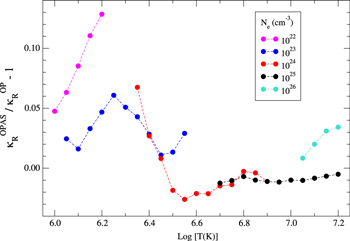
Standard image High-resolution imageWe compared OPAS Rosseland opacities to OP data (http://cdsweb.u-strasbg.fr/topbase/topbase.html). Comparisons have been performed for integer values of ![$\mathrm{log}[{N}_{{\rm{e}}}({\mathrm{cm}}^{-3})]$](https://content.cld.iop.org/journals/0067-0049/220/1/2/revision1/apjs518027ieqn108.gif) in the range
in the range ![$[22,26]$](https://content.cld.iop.org/journals/0067-0049/220/1/2/revision1/apjs518027ieqn109.gif) and for
and for ![$\mathrm{log}[T({\rm{K}})]$](https://content.cld.iop.org/journals/0067-0049/220/1/2/revision1/apjs518027ieqn110.gif) between 6 and 7.2. Expressed as
between 6 and 7.2. Expressed as  , the differences are shown in Figure 6 for
  . The OPAS and OP calculations are in good agreement, except at the lower electron density where OPAS data are up to
  . The largest difference is obtained for
 ![$\mathrm{log}[{N}_{{\rm{e}}}({\mathrm{cm}}^{-3})]=22$](https://content.cld.iop.org/journals/0067-0049/220/1/2/revision1/apjs518027ieqn114.gif) and
and ![$\mathrm{log}[T({\rm{K}})]=6.2$](https://content.cld.iop.org/journals/0067-0049/220/1/2/revision1/apjs518027ieqn115.gif) . For these thermodynamical conditions, our calculations indicate that Cl, K, and Ti (three elements which are not included in the OP database) contribute together for 1% to the mixture Rosseland opacity. The analysis of the remaining
. For these thermodynamical conditions, our calculations indicate that Cl, K, and Ti (three elements which are not included in the OP database) contribute together for 1% to the mixture Rosseland opacity. The analysis of the remaining  difference is complicated because eight metallic elements (C, N, O, Si, S, Ar, Ca, and Fe) noticeably contribute. Oxygen and iron are the major metallic contributors (20% and 12% to the total opacity, respectively). Focusing on iron, the individual contribution we calculated is 40% higher than the value deduced from OP data. OPAS and OP iron average ionization are very close (16.10 and 16.06, respectively) and the charge state distributions are in good agreement. In the photon energy range where L-shell photoexcitation processes are prevalent, the OP spectrum exhibits deep gaps between the main resonant structures. The OPAS calculation involves an exhaustive sampling of excited atomic states. Bound-bound transitions from these states mainly contribute to reduce the gaps compared to the OP calculation. Furthermore, the use of statistical ionic Stark broadening in OPAS calculations enhances the gap filling efficiency near the L-shell photoionization threshold.
Figure 6. Comparison of OPAS Rosseland opacities to OP data expressed as  for various Ne values (AGS'09 composition,
  ).
).
Download figure:
Standard image High-resolution image
6. CONCLUSION
According to the AGS'09 composition (Asplund et al. 2009), the OPAS opacity model has been used to calculate opacities of stellar plasmas in local thermodynamic equilibrium. Dedicated to solar interior modeling, calculations have been performed for temperatures between ![$\mathrm{log}[T({\rm{K}})]=6$](https://content.cld.iop.org/journals/0067-0049/220/1/2/revision1/apjs518027ieqn119.gif) and
and ![$\mathrm{log}[T({\rm{K}})]=7.2$](https://content.cld.iop.org/journals/0067-0049/220/1/2/revision1/apjs518027ieqn120.gif) , and for electron densities between
, and for electron densities between  and
and  . Possible sources of uncertainty in the tabulations have been examined, and the associated precision has been estimated to be approximately 1%. Twenty-two chemical element mixture Rosseland opacities have been tabulated for various hydrogen and metallic element mass fractions. Comparisons with the OPAL and OP data have shown a good agreement, except in the low-temperature and low-density domain where the OPAS results are up to approximately
  larger.
This work has been performed under the auspice of the Agence Nationale de la Recherche (Contract No. ANR-12-BS05-0017 entitled OPACITY). The authors thank Sylvaine Turck-Chièze for having stimulated this work.