

Abstract
This article reviews how nuclear fission is described within nuclear density functional theory. A distinction should be made between spontaneous fission, where half-lives are the main observables and quantum tunnelling the essential concept, and induced fission, where the focus is on fragment properties and explicitly time-dependent approaches are often invoked. Overall, the cornerstone of the density functional theory approach to fission is the energy density functional formalism. The basic tenets of this method, including some well-known tools such as the Hartree–Fock–Bogoliubov (HFB) theory, effective two-body nuclear potentials such as the Skyrme and Gogny force, finite-temperature extensions and beyond mean-field corrections, are presented succinctly. The energy density functional approach is often combined with the hypothesis that the time-scale of the large amplitude collective motion driving the system to fission is slow compared to typical time-scales of nucleons inside the nucleus. In practice, this hypothesis of adiabaticity is implemented by introducing (a few) collective variables and mapping out the many-body Schrödinger equation into a collective Schrödinger-like equation for the nuclear wave-packet. The region of the collective space where the system transitions from one nucleus to two (or more) fragments defines what are called the scission configurations. The inertia tensor that enters the kinetic energy term of the collective Schrödinger-like equation is one of the most essential ingredients of the theory, since it includes the response of the system to small changes in the collective variables. For this reason, the two main approximations used to compute this inertia tensor, the adiabatic time-dependent HFB and the generator coordinate method, are presented in detail, both in their general formulation and in their most common approximations. The collective inertia tensor enters also the Wentzel–Kramers–Brillouin (WKB) formula used to extract spontaneous fission half-lives from multi-dimensional quantum tunnelling probabilities (For the sake of completeness, other approaches to tunnelling based on functional integrals are also briefly discussed, although there are very few applications.) It is also an important component of some of the time-dependent methods that have been used in fission studies. Concerning the latter, both the semi-classical approaches to time-dependent nuclear dynamics and more microscopic theories involving explicit quantum-many-body methods are presented. One of the hallmarks of the microscopic theory of fission is the tremendous amount of computing needed for practical applications. In particular, the successful implementation of the theories presented in this article requires a very precise numerical resolution of the HFB equations for large values of the collective variables. This aspect is often overlooked, and several sections are devoted to discussing the resolution of the HFB equations, especially in the context of very deformed nuclear shapes. In particular, the numerical precision and iterative methods employed to obtain the HFB solution are documented in detail. Finally, a selection of the most recent and representative results obtained for both spontaneous and induced fission is presented, with the goal of emphasizing the coherence of the microscopic approaches employed. Although impressive progress has been achieved over the last two decades to understand fission microscopically, much work remains to be done. Several possible lines of research are outlined in the conclusion.
Export citation and abstract BibTeX RIS
1. Introduction
Experiments on the bombardment of Uranium atoms (charge number Z = 92) with neutrons performed by Hahn and Strassmann in 1938–1939 and published in [1, 2] showed that lighter elements akin to Barium (Z = 56) were formed in the reaction. In February 1939, this observation was explained qualitatively by Meitner and Frisch in [3] as caused by the disintegration of the heavy Uranium element into lighter fragments. This tentative explanation was based on the liquid drop model of the nucleus that had been introduced a few years earlier in [4] by Bohr. A few months after these results N. Bohr himself, together with Wheeler, formalized and quantified Meitner's arguments in their seminal paper [5]. They described fission as the process during which an atomic nucleus can deform itself up to the splitting point as a result of the competition between the nuclear surface tension that favours compact spherical shapes and the Coulomb repulsion among protons that favour very elongated shapes to decrease the repulsion energy. They introduced the concepts of compound nucleus, saddle point (the critical deformation beyond which the nuclear liquid drop is unstable against fission) and fissility (which captures the ability of a given nucleus to undergo fission), provided estimates of the energy release during the process, of the dependence of the fission cross-section on the energy of incident particles, etc. Although tremendous progress has been made since 1939 in our understanding of nuclear fission, many of the concepts introduced by Bohr and Wheeler remain very pertinent even today.
1.1. Fission in science and applications
In simple terms, nuclear fission is the process during which an atomic nucleus made of Z protons and N neutrons (A = N + Z) may split into two or more lighter elements. The nuclear 'fissility' parameter, given by  with I =(N − Z)/A and
  , is a convenient quantity to characterize the ability of a nucleus to fission as suggested in [6–8]. In the liquid drop model, the fissility is related to the ratio between the Coulomb and surface energy of the drop. For values of x > 1, the drop is unstable against fission, and nuclear fission can then occur spontaneously. This is the case, for instance, in heavy nuclei with large Z values such as actinides or transactinides. The process is characterized by the spontaneous fission half-life
  , which is the time it takes for half the population of a sample to undergo fission. Fission can also be induced through a nuclear reaction of a target nucleus with projectiles such as neutrons, protons, alpha particles or gamma rays ('photofission'). There are four well known cases (239, 241Pu and 233, 235U) where the absorption of a neutron in thermal equilibrium with the environment—with kinetic energy of a few tens of meV—is sufficient to trigger fission ('fissile elements'). Note that 235U is the only such fissile element that is naturally occurring on earth.
Since the fissility parameter increases quadratically with Z, spontaneous fission is one of the most important limiting mechanisms to the existence of superheavy elements and is discussed in specialized review articles such as [9, 10], as well as in several textbooks [11, 12]. Theoretical studies of the location of the next island of stability beyond Lead are, therefore, largely focused on the accurate determination of spontaneous fission half-lives; see for instance the following papers [13–20].
Nuclear fission also plays an important role in the formation of elements in the rapid neutron capture process (r-process) of nucleosynthesis in stellar environments. Modern simulations of neutron star–neutron star or neutron star–black hole mergers performed in [21–23] suggest a vigorous r-process with fission recycling. In a fission recycling scenario, the nucleosynthesis flow proceeds beyond the N = 126 closed shell to the region where neutron-induced, β-delayed, or spontaneous fission becomes likely. The fission products rejoin the r-process flow at lower A, continuing to capture neutrons until again reaching the fission region. Fission recycling is thus expected to contribute to the abundance pattern between the second ( ) and third r-process (
 ) peaks. This appears consistent with observations of the r-process-enhanced halo stars—unusual old, metal-poor stars at the edges of our galaxy that contain r-process elements in quantities measurable via high-resolution spectroscopy. Most of the relatively complete 56 < Z < 82 patterns observed in these stars are strikingly similar and a good match to the solar r-process residuals within this element range as reported in [24, 25].
Because of the strong nuclear binding, the energy released during fission is very large (compared to other energy production sources), typically of the order of 200 MeV per fission event. Most of it is kinetic energy of the fission fragments while about 10–20% of it is excitation energy. In a typical fission process, the formation of the fission fragments will thus be accompanied by neutron and gamma emission. In a nuclear reactor, these neutrons can be reabsorbed by the fissile elements present in the core, thereby triggering new fission events. The magnitude of this chain reaction can be controlled by neutron absorbers. Clearly, all characteristics of the fission process are essential to understanding the physics behind the technology required for efficient, reliable and safe nuclear technology applications. For instance, understanding the mechanism of induced fission at the level of making reliable prediction in regions where no experimental data is available will be of paramount importance in technological applications.
1.2. Defining a microscopic theory of nuclear fission
In this review, the term 'microscopic theory' should be understood as pertaining to the methods and concepts of nuclear density functional theory (DFT)—in its broadest sense. In particular, we will use interchangeably the expression of DFT and self-consistent mean field (SCMF) theory. Extensions beyond mean field theory—such as, for example, projection or configuration mixing techniques—will also be generously included under the DFT label. The choice of this loose definition stems from the need to clearly differentiate current microscopic approaches to fission from configuration interaction methods such as ab initio techniques or the nuclear shell model. It is also a reminder that the basic concepts and approximations essential in the theoretical description of fission are to a large extent independent of the formal differences between the SCMF and DFT.
The overall framework of the microscopic theory of fission based on DFT/SCMF is summarized in figure 1. The starting point is to view the nucleus as a system of protons and neutrons, treated as point-like particles, in interaction. We further assume that the ground-state of the system can be well approximated by a symmetry-breaking quasiparticle vacuum. As a result of this approximation, the two basic degrees of freedom of the theory are the one-body density matrix ρ and the pairing tensor κ. These objects are determined by solving the Hartree–Fock–Bogoliubov (HFB) equation, also known as Bogoliubov–de Gennes equation in condensed matter. The Wick theorem allows computing the expectation value of any operator based solely on the knowledge of the density matrix and pairing tensor. These concepts are briefly summarized in section 2.2.1.

Figure 1. Schematic workflow of the microscopic theory of fission based on nuclear density functional theory.
Download figure:
Standard image High-resolution imageAt the HFB approximation, the energy of the nucleus is a functional of ρ and κ. In the particular case of the self-consistent mean field, this functional is in fact derived from the expectation value of an effective nuclear Hamiltonian  on a quasiparticle vacuum; in the DFT picture, the energy density functional (EDF) is not necessarily related to any Hamiltonian. In both cases, the form of the EDF should in principle be constrained by our knowledge of nuclear forces. However, the various parameters that enter the definition of the EDF are typically readjusted to data in nuclear matter and finite nuclei to account for the HFB approximation. The Skyrme and Gogny forces are among the two most popular effective nuclear potentials that have been used, among others, in fission studies. The characteristics of the nuclear EDF, including a short discussion of how their parameters are adjusted to data, are presented in section 2.2.3.
Allowing for spontaneous breaking of the symmetries of the nuclear force at the level of the quasiparticle vacuum is reminiscent of the historical picture of fission: if the one-body density matrix is not rotationally invariant, its spatial distribution represents a deformed nuclear shape. Fission can then be viewed as a process during which the deformation becomes so large that two separate fragments appear. This viewpoint can be formalized by introducing a set of collective variables that represent the motion of the nucleus as a whole and control the fission process. The characteristics of the resulting potential energy surface (PES), i.e. the energy as a function of the chosen collective variables, determines fission properties. For example, differences in the characteristics of potential energy barriers of nuclei qualitatively explain the range of spontaneous fission half-lives observed experimentally. In neutron-induced fission, the time 'from saddle to scission', which is the time it takes for the nucleus to go from the top of the highest barrier to a configuration with two separated fragments, is also strongly dependent on the characteristics of the PES.
In the adiabatic approximation, it is further assumed that there is a perfect decoupling between the motion in collective space and the intrinsic motion of individual nucleons. This hypothesis originates from the observation that the time from saddle to scission is typically of the order of 10−19 s. This is about two orders of magnitude slower than the time scale that can be inferred from the average binding energy per nucleon ( MeV). As a result, one can explore the collective space by seeking solutions to the HFB equations that yield specific values of the collective variables: this is how potential energy surfaces are computed in practice. Section 2.3 discusses the role of various collective variables in fission; see also section 2.1.1 for geometrical parametrizations of the nuclear surface used in semi-phenomenological approaches.
For specific values of the collective variables, the density of nucleons  may exhibit two disconnected regions of space with a high density of particles. Such a configuration corresponds to separated fragments. The frontier between configurations associated to the whole compound nucleus and those associated with the fission fragments is called the scission line; in N-dimensional collective spaces, it is in fact an N − 1-dimensional hyper-surface. The actual definition of scission is ambiguous and is discussed in detail in section 2.4. In non-adiabatic approaches to fission such as time-dependent density functional theory (TDDFT), scission occurs 'naturally' from the competition between short-range nuclear forces and Coulomb repulsion as the system is being evolved in time from some initial state (usually some specific quasiparticle vacuum). In the adiabatic approximation, however, there is no such 'dynamical' mechanism to simulate the evolution of the system.
1.3. Challenges for a predictive theory of fission
As briefly mentioned in the previous section, there are different forms of nuclear fission, and the relevant observables that theorists need to compute thus differ depending on the mechanism under study.
- Spontaneous fission (SF) is mostly characterized by the fission half-lives
 , which range from 4.2 μs in 250No to over 1.4 1010 years for 232Th, or a range of over 35 orders of magnitude. The characteristics of the fission fragments are also important for astrophysical applications, or for establishing benchmark data for nuclear material counting techniques used, e.g. in international safeguards, see for instance [26].
 - In neutron-induced or photofission reactions, the focus is more on the fission fragments. The relevant observables are thus the charge and mass distributions of the fragments; their total kinetic (TKE) and excitation energy (TXE) distributions, the average number of neutrons emitted from each fragment and the average neutron energy; the average gamma multiplicity (i.e. number of gamma rays emitted) per fragment and the average gamma ray energy, etc. All these observables should be computed as a function of the energy of the incident particle (neutron or photon). Applications of induced fission in energy production typically require accuracy of less than a 1% on these quantities.
- In β-delayed fission, the compound nucleus has been itself produced by β decay. The probability and characteristics of the subsequent fission will be dependent on the excited spectrum of the compound nucleus, and of the β-decay process itself. Calculating β-decay rates is, in itself, particularly challenging for nuclear DFT, since it is dependent on detailed knowledge of the nuclear wave-function. Until now, there have been no attempt at computing β-delayed fission rates in a fully microscopic setting.


This variety of observables imposes various constraints on theory. For example, the description of neutron-induced fission with fast neutrons ( MeV) requires accurate modelling of the compound nucleus up to excitation energies of 20 MeV or so; predictions of spontaneous fission half-lives in superheavy nuclei are contingent on the predictive power of nuclear EDF far from stability; β-delayed fission rates depend on a quantitatively accurate description of weak processes in nuclei, etc.
Over the past decade, nuclear DFT has made great strides toward becoming a predictive tool for nuclear structure; see [27] for a description of a comprehensive effort to build a universal energy functional. In particular, there is little doubt today that the theoretical framework outlined in the previous section and explained in greater detail in sections 2 and 3 is sufficient to explain, at the very least semi-quantitatively, multiple aspects of the fission process—from the trend of fission half-lives along isotopic lines via the shape of fission fragment mass distributions to the overall properties of fission fragments; see section 5 for an overview of recent results. The main question, therefore, is whether this framework can deliver the accuracy and precision required in applications—be it to answer fundamental science questions or provide parameter-free input for nuclear technology.
Reaching such a goal will require progress on at least three fronts:
- At the most fundamental level, DFT predictions always depend on the intrinsic quality of the nuclear EDF. Currently, all EDFs used so far in fission studies have been based on phenomenological potentials such as the Skyrme and Gogny force. While these potentials have been essential in demonstrating the validity of the microscopic approach, there is a large consensus in the nuclear theory community that potentials with a much sounder connection to the theory of nuclear forces should be developed. How exactly to do this remains an open question.
- On a more technical note, applications of DFT to fission are still limited by a number of approximations. In current adiabatic approaches, the solution to the nuclear many-body problem is obtained only for the lowest energy state and the number of collective variables is rather small; in current non-adiabatic time-dependent approaches, tunnelling is not possible, important correlations such as pairing are often modelled approximately and only one-body dissipation is taken into account. In both cases, open channels (particle evaporation, gamma emission) are rarely taken into account at the same level of detail.
- Finally, one should emphasize that the physics of scission remains poorly known. How fission fragments acquire their identity, and the connection of this process with the physics of quantum entanglement, has not been studied.
Although this article tries to provide as complete as possible a review of the current microscopic theory of fission, choices had to be made. First, we only mention topics where results were obtained with a DFT approach, and voluntarily leave out all the other areas where this is not the case. For example, we do not discuss the phenomenon of ternary fission observed in the spontaneous fission of actinides such as in [28]; the generation of angular momentum in the fission fragments discussed, e.g. in [29] and references therein; or the very complex problem of the fission spectrum (identifying the characteristics of the neutron, γ and β-decay emitted during fission); see [30] for a recent discussion of the state of the art. In view of these considerations, our most controversial choice is certainly to leave out results obtained with the relativistic formulation of DFT (called relativistic mean-field or covariant density functional theory) reviewed in [31, 32]. This was motivated partly by the need to keep the length of this article reasonable, but also by the fact that most of the methods discussed in the non-relativistic framework can easily be ported to the relativistic one. There are excellent articles on fission within various versions of covariant density functional theory, and we refer, e.g. to [14, 18, 33–40] for a short sample of the existing literature.
2. Potential energy surfaces
As mentioned in the introduction, the hypothesis of adiabaticity has played a special role in the theory of fission since its introduction by Niels Bohr back in his 1939 paper [5]. The notion that a small set of collective degrees of freedom was sufficient to describe most of the physics of fission has proved extraordinarily fruitful in semi-phenomenological approaches [9, 41, 42]. It is no surprise, therefore, that the same concept has been adapted to a more microscopic theory based on nuclear density functional theory (DFT).
The cornerstone of the implementation of the adiabatic approximation in fission theory is the definition of a potential energy surface (PES) in an arbitrary collective space. This PES is the analogue of the classical phase space of Lagrangian and Hamiltonian mechanics. In all the current approaches to fission that rely on the adiabatic approximation, the first step is, therefore, to define the most relevant collective variables and compute the PES.
In section 2.1, we briefly recall how this is done in macroscopic-microscopic methods, which are often an invaluable source of inspiration for density functional theory. In the latter, the PES is computed by solving the DFT equations, which take the form of the Hartree–Fock–Bogoliubov (HFB) equations. Section 2.2 gives a modern presentation of the energy density functional (EDF) implementation of DFT. This includes a reminder about the HFB theory in section 2.2.1 and of its BCS approximation in section 2.2.2; an overview of the main components of standard energy functionals in section 2.2.3; a foray into how to compute PES at high excitation energies in section 2.2.4; a list of the most important 'dynamical' corrections to the PES in section 2.2.5. The large choice of possible collective variables, including either geometric or non-geometric quantities, is discussed in section 2.3. Finally, we review the various criteria that have been introduced in the literature to define the scission configurations in section 2.4.
2.1. The macroscopic-microscopic approach
Starting with the pioneering work of Bohr and Wheeler, many theoretical studies of fission have been performed with empirical models derived from the liquid drop formula; see [9, 41] for comprehensive reviews. The introduction of the shell correction method by Strutinsky and collaborators in the nineteen sixties was essential to providing more microscopic insight to this approach and accounting for the role of nucleon degrees of freedom and of (some) features of nuclear forces. In the early nineteen seventies, the macroscopic-microscopic (MM) method was already well established and had been successfully applied to the problem of nuclear fission as exemplified in [8, 9]. Since then, it has remained a popular and effective way to perform large scale studies of nuclear properties in general ([43–46]) and fission in particular ([47–49]). Although this review is devoted to the microscopic theory of fission, it is not out of place to recall some of the most important features of the MM approach, since DFT has borrowed many of its most successful concepts.
In simple terms, the MM approach consists in viewing the nucleus as a finite chunk of nuclear matter, the energy of which is parametrized as a function of the charge, mass and deformations  of the nucleus. The total energy of the nucleus is decomposed as a sum of three terms: (i) a macroscopic energy
  that is often approximated by a deformed liquid drop or droplet formula and represents bulk nuclear properties, see the work by Myers and Swiatecki in [50–52] for a complete description of this term. In the language of second quantization, this is essentially a zero-body term; (ii) a shell correction
  that accounts for the distribution of single particle levels in the average nuclear potential and thus has a one-body origin; (iii) a pairing correction
  , which has a two-body origin. The total energy thus reads formally

where  represents the set of all deformations characterizing the nuclear surface. The formalism has also been extended to account for finite angular momentum, e.g. in [11, 44], and intrinsic excitation energy, for instance in [53, 54].
2.1.1. Parametrization of the nuclear surface.
In the MM approach, the energy (1) is a function of all the parameters needed to describe the nuclear shape. In other words, the nuclear surface must be parametrized explicitly. Numerous parametrizations have been introduced over the years; see [55] for a comprehensive review. In this section, we wish to recall some of the most common parametrizations, especially those that have been introduced to describe extremely deformed nuclear shapes near scission.
The simplest and most common parametrization is based on the multipole expansion of the nuclear radius [56],

where  is a parametrization of the nuclear radius for a spherical nucleus of mass A (
 fm);
fm);  is a factor accounting for the conservation of nuclear volume with deformation; the
  are the deformation parameters; and
  are the usual spherical harmonics. This parametrization of the nuclear surface is ideal for small to moderate deformations. However, a well-known problem of this formulation discussed in [57, 58] is that it does not provide a unique representation of the nuclear surface. In addition, the number of active deformation parameters needed to characterize very elongated shapes can become large. These difficulties also manifest themselves in the DFT framework since, as we will discuss in section 2.3.1, the collective variables most commonly used are the mass multipole moments of the nucleus, which are closely related to the spherical harmonics of (2). For illustration, we show in figure 2 a cross-section of the shapes obtained with the expansion (2) for the nucleus 240Pu with
  and
and  .
.

Figure 2. Axial shapes obtained with the expansion (2) of the nuclear radius for  (plain curve),
  (dashed curve) and
  (dashed–dotted curve). For each curve, all other deformation parameters are 0.
Download figure:
Standard image High-resolution imageBecause of the limitations of expansion (2), alternative parametrizations of the nuclear surface have been advocated over the years. One of the most popular is the Funny Hills shapes of [9]. Assuming axial symmetry along the z-axis of the intrinsic reference frame, a point on the surface is characterized by the usual cylindrical coordinates  . In this case, the distance ρ from the nuclear surface to the axis of symmetry is given by


where A, B, and α are the parameters characterizing the shape; c is related to the elongation of the system, and defines the dimensionless variable  ; in practice, A is obtained from the volume conservation condition, and the parameter B is substituted by another,
  , which is related to the thickness of the neck. Therefore, the Funny Hills parametrization is most commonly characterized by the set
  . The figure 3 illustrates the shapes obtained for
  (top panel) and
  (bottom panel), each case with c varying between 1.0 and 2.2 by step of 0.3.

Figure 3. Funny Hills parametrization of nuclear shapes for  (top panel) and
  (bottom panel). c varies from 1.0 to 2.2 by step of 0.3.
Download figure:
Standard image High-resolution imageAn alternative to the Funny Hills parametrization is the one proposed by the Los Alamos group in [7]. It also applies to axially-symmetric shapes. In cylindrical coordinates, the nuclear surface is described by three quadratic surfaces of revolution

The nine parameters  are not all independent: the condition of volume conservation eliminates one parameter; the condition of continuity and differentiability of the surface at the two interfaces z1 and z2 eliminate two more parameters; fixing the centre of mass of the shape can also eliminate an additional parameter, so that only five independent parameters are ultimately needed. They are denoted
  and correspond respectively to the elongation of the whole nucleus, the mass asymmetry of the two nascent fragments, the axial quadrupole deformation of the left and right fragment, and the thickness of the neck; see [49] for details and derivations.
The last category of nuclear shape parametrization originally introduced in [59] is based on Cassini ovals. The general expression for Cassini ovals is

with a and b the only parameters. If a = 0, then the shape reduces to a sphere of radius b; if a > b (6) represents two separate fragments. When using this parametrization to represent the nuclear shape, the volume conservation condition allows eliminating one of the two parameters. Therefore, Cassini ovals represent a single-parameter parametrization of the nucleus that can reproduce shapes from the spherical point to two distinct fragments separated by an arbitrary distance. To account for mass asymmetry, Cassini ovals can be distorted by substituting  in the left-hand side of (6). The figure 4 illustrates some of the typical shapes obtained in the symmetric case of (6).

Figure 4. Axial shapes obtained with the parametrization (6) for u = 0.0, 0.4, 0.8, 1.0, 1.2. The case u = 0 corresponds to the sphere, the case u = 1.0 to the scission point and the case u = 1.2 to the two separated fragments.
Download figure:
Standard image High-resolution imageOnce a parametrization of the nuclear surface has been established, the macroscopic part of the energy  can be computed. In the most advanced parametrization of the macroscopic energy, the surface, surface-symmetry, Coulomb and Wigner terms depend on the deformation via geometrical form factors that can be computed in a straightforward manner when the nuclear shape is known. The other terms are deformation-independent and adjusted to global nuclear properties [50–52].
2.1.2. Quantum corrections.
In addition to the macroscopic energy, the MM approach relies on various quantum corrections. Here, the adjective 'quantum' recalls the fact that these corrections can only be computed by solving the Schrödinger equation of quantum mechanics.
The shell correction is the most important correction. It was introduced in [60] in order to account for the single particle shell structure in the calculation of the total energy. The starting point of the method is a phenomenological nuclear potential  including a central part such as e.g. the Nilsson, Woods–Saxon or folded-Yukawa potential, a spin–orbit potential and the Coulomb potential for protons. The geometry of these potentials should be consistent with that of the nuclear surface: in the case of the Woods–Saxon or folded-Yukawa potential, this implies that the various terms depend on the distance of the current point to the nuclear surface, parametrized as discussed in the previous section. Given the potential and its deformation, one solves the one-body Schrödinger equation in order to obtain the (deformed) single particle energies en and wave functions
  . The last step is to approximate the discrete sequence of states
  by a continuous distribution
  following the Strutinsky averaging procedure. The shell correction is then defined as

In the last expression, the shell correction should be computed for both protons and neutrons; the summation extends either over the Z and N lowest orbitals (ground-state) or over a subset of orbitals (excited states). In addition to providing a more realistic estimate of binding energies, the introduction of a one-body potential has given birth to a very powerful phenomenology based on single particle orbitals as basic degrees of freedom of nuclei; see [11] for a reference textbook on this topic.
Pairing correlations are incorporated into the MM approach in the form of an average pairing energy in the macroscopic energy  supplemented by a pairing energy correction. The average pairing energy does not contribute to fission (it is independent of the deformation), while the pairing energy correction is treated in a very similar manner to shell effects. The solution to the BCS equations define the pairing correlation energy
  . Assuming again a continuous level distribution, one can define a smooth pairing energy
  . The difference
  defines the pairing correction energy. In most applications to fission, pairing is described within the BCS theory with schematic interactions such as a constant seniority pairing force. Particle number conservation can be accounted for exactly by projection techniques as described in [61] or approximately through the Lipkin–Nogami prescription, see application in [8, 43]. Such a scheme was applied extensively in the fission studies by the LANL/LBNL and Warsaw groups, see, e.g. [48, 49, 62–66] and references therein for some recent work.
2.2. The energy density functional formalism
The energy density functional (EDF) formalism at the heart of the current microscopic theory of fission is the implementation of DFT in the particular context of atomic nuclei. Let us briefly recall that the DFT used in electronic structure theory relies on the rigorous existence theorems of Hohenberg and Kohn [67]. It begins with the expression of the energy of the system as a functional of the local electron density  . The density is determined in practice by solving the Kohn–Sham equations—formally analogue to the Hartree equations [68]. Note that various extensions of the Hohenberg–Kohn theorem to handle exchange terms exactly, excited states, systems at finite temperature, and superfluid correlations are also available; see [69, 70] for a detailed presentation. In these extensions, the Kohn–Sham scheme is reformulated starting, e.g. from the full one-body density matrix for the exact treatment of exchange terms [71].
In nuclear physics, the true Hamiltonian is not known, nuclei are self-bound, and, as emphasized in [72], correlation effects are much stronger than in electron systems. Also, pairing correlations play a special role, which is reflected by the importance of the Bogoliubov transformation in nuclear structure. There have been various attempts to extend the Hohenberg–Kohn theorem to self-bound systems characterized by their intrinsic density (defined in the centre of mass reference frame), see discussions in [73–78]. However, the resulting Kohn–Sham scheme does not seem to be as simple as in electronic DFT as shown in [73, 74]. In addition, how to rigorously include symmetry-breaking effects (and subsequently restore these symmetries) in such schemes remains an open question.
Historically, most nuclear energy functionals have been explicitly derived from the expectation value of an effective nuclear Hamiltonian on a quasiparticle vacuum leading to the notion of self-consistent nuclear mean field reviewed in details in [79]. In the spirit of the Hohenberg–Kohn theorem, the SCMF is equivalent to expressing the energy as a functional of the intrinsic, one-body, non-local density matrix ρ and non-local pairing tensor κ. In addition, these objects may break many of the symmetries of realistic nuclear forces such as translational or rotational invariance, parity, time-reversal invariance, and particle number. This spontaneous symmetry breaking is essential for introducing long-range correlations in the nuclear wave function as discussed in [61, 80]. In the coming sections, we recall some of the basic features of the nuclear EDF approach. We begin with the Hartree–Fock–Bogoliubov (HFB) theory in section 2.2.1, followed by its BCS approximation in section 2.2.2; in section 2.2.3, we give a brief survey of standard energy functionals; we then introduce the finite temperature formalism in section 2.2.4 as a method to describe excited states; finally, we list in section 2.2.5 the various corrections to the energy that have a beyond mean-field origin.
2.2.1. Self-consistent Hartree–Fock–Bogoliubov theory.
The HFB approximation to the energy is centred on the Bogoliubov transformation defining quasiparticle creation and annihilation operators in terms of a given single particle basis  of a (restricted) Fock space


While the Hilbert space of single particle wave functions is infinite, in practice summations are truncated up to a maximum basis state N. It is convenient to introduce a block matrix notation and matrices of double dimension by writing the equation above as

which defines the matrix W of the Bogoliubov transformation

The quasiparticle operators must satisfy canonical fermion commutation relations, which can be summarized by the condition

with IN the N-dimensional identity matrix. The HFB wave function  is defined as the vacuum of the quasiparticle annihilation operators,
  for all μ. This leads to writing
  where
where  is the particle vacuum of Fock space and the product runs over all the μ indexes that render
  non zero.
Densities.
If the ground-state wave function takes the form of a Bogoliubov vacuum, the Wick theorem guarantees that the basic degrees of freedom are the one-body density matrix ρ, the pairing tensor κ and its complex conjugate  [61, 81]. Each of these objects can be expressed as a function of the Bogoliubov transformation,

The notation can be further condensed by introducing the generalized density matrix,

which is given in terms of the W matrix of the Bogoliubov transformation and the matrix of quasiparticle contractions

as  . The generalized density matrix encapsulates in a single matrix all degrees of freedom of the theory and simplifies the formal manipulations required in the application of the variational least energy principle.
Variational principle.
Since ρ, κ and  are the only degrees of freedom, the energy can be expressed most generally as the functional
 ![$E\left[\rho,\kappa,{{\kappa}^{\ast}}\right]\equiv E\left[\mathcal{R}\right]$](https://content.cld.iop.org/journals/0034-4885/79/11/116301/revision1/ropaa353dieqn057.gif) . In practice, one often distinguishes between the particle–hole and particle–particle channel,
. In practice, one often distinguishes between the particle–hole and particle–particle channel,

although the distinction is a bit artificial since ρ and κ are related through  . Please also note that pairing interactions depending on the density ρ are very popular in nuclear physics, which adds an extra dependence in
  . The actual matrix
  is obtained by minimizing the energy under the condition that the HFB solution remains a quasiparticle vacuum, which is equivalent to
  . We thus have to minimize

where  is a matrix of (undetermined) constraints. In this expression and the rest of this paper, 'tr' refers to the trace in the single particle basis (possibly doubled). The variations of the energy are given by

Since  , we find after some simple algebra,

Let us denote  . In matrix form, the condition that the variations of the energy should be zero is expressed by the equation

Pre- and post-multiplying this equation by  and subtracting the results after noticing that
  , we find the final form of the HFB equation

Since  , we have by definition
 . Considering the form (14) of the generalized density, we find that the matrix of
  reads
reads

with the mean field h and pairing field  defined by

The form of the HFB equation (21) is not well suited for its practical solution and, therefore, it is often reinterpreted by considering that ![$\left[\mathcal{H},\mathcal{R}\right]=0$](https://content.cld.iop.org/journals/0034-4885/79/11/116301/revision1/ropaa353dieqn072.gif) implies that
implies that  and
and  can be diagonalized by the same Bogoliubov transformation. Since the generalized density matrix is diagonalized by W as shown in (15), the same must hold for
  ,
,

This represents a non-linear diagonalization problem (since  depends upon W through the densities) with eigenvalues
  and eigenvectors W. It turns out that the matrix of eigenvalues can be written schematically

that is, for each positive eigenvalue  , there is another one of opposite sign
  . The eigenvalues of the HFB matrix are referred to as 'quasiparticle energies'. In section 4.1 p 33, we discuss the technical aspects of solving such a non-linear eigenvalue problem. The quasiparticle energies
  defined above should not be confused with the single particle energies typical of the phenomenological mean field potentials of the MM method. The equivalent to the single particle energies in the HFB case are the eigenvalues of the Hartree–Fock (HF) Hamiltonian h of (23). The study of those quantities allows obtaining the same degree of insight that can be obtained by the study of the Nilsson orbitals.
Energy and fields.
In nuclear physics, the energy functional ![$E\left[\rho,\kappa,{{\kappa}^{\ast}}\right]$](https://content.cld.iop.org/journals/0034-4885/79/11/116301/revision1/ropaa353dieqn081.gif) is typically composed of two parts: one is derived from an effective two-body Hamiltonian,
is typically composed of two parts: one is derived from an effective two-body Hamiltonian,

where tij refers to the matrix elements of the one-body kinetic energy operator and  to the anti-symmetrized matrix elements of the two-body potential. The other part of the energy functional comes in the form of various phenomenological density dependent terms that have to be handled with some care as they introduce additional terms in the HF Hamiltonian and pairing fields that come in the form of rearrangement potentials (see below). In the case of such an effective two-body Hamiltonian, the HFB energy is simply given by
  , with
  the quasiparticle vacuum introduced earlier. Considering the definitions (13) for the density matrix and pairing tensor, the application of the Wick theorem gives

In this particular case, the mean field potential and the pairing field are given as a function of the two-body matrix elements by

and the HF Hamiltonian reads  . The notation can be further condensed by defining the generalized kinetic energy and mean field matrices by

With these notations, we note that ![$\mathcal{H}\left[\mathcal{R}\right]=\mathcal{T}+\mathcal{K}\left[\mathcal{R}\right]$](https://content.cld.iop.org/journals/0034-4885/79/11/116301/revision1/ropaa353dieqn086.gif) . The total energy can then be written in the very compact form
. The total energy can then be written in the very compact form

with

Density-dependent interactions.
In the practical implementation of the HFB theory in nuclear structure, special attention should be paid to the very common case of two-body, density-dependent effective 'forces' ![${{\hat{v}}^{\text{DD}}}\left(\boldsymbol{r},\boldsymbol{r}^{{\prime}}\right)={{\hat{v}}^{\text{DD}}}\left[\rho \left(\boldsymbol{R}\right)\right]\delta \left(\boldsymbol{r}-\boldsymbol{r}^{{\prime}}\right)$](https://content.cld.iop.org/journals/0034-4885/79/11/116301/revision1/ropaa353dieqn087.gif) with
with  . Note that in this case, the potential
  cannot be put into strict second quantized form—as emphasized in [82]. However, one can still define an energy functional
 ![$E\left[\rho,\kappa,{{\kappa}^{\ast}}\right]$](https://content.cld.iop.org/journals/0034-4885/79/11/116301/revision1/ropaa353dieqn090.gif) by taking the expectation value of
by taking the expectation value of  in coordinate space on a quasiparticle vacuum. Given the energy functional, the mean field and pairing field can then be defined from (23). When computing these derivatives with respect to the density matrix, additional contributions related to the matrix elements of
  will arise (rearrangement terms). They have the generic form

with

Note that one could also consider pairing-tensor-dependent potentials in the same way. Recently, an extension of the above scheme so as to consider finite range density-dependent forces has been proposed [83]. In this case, the simple formulas above have to be adapted but the same conceptual procedure remains valid.
Representation based on the Thouless theorem.
There is an alternative way to obtain and represent the HFB equation, which is based on the Thouless theorem of [84]. We recall that the Thouless theorem presented, e.g. in [61, 81], establishes that two non-orthogonal quasiparticle vacua  and
and  (corresponding to two different Bogoliubov transformations W0 and W1) are related through

where  is an hermitian one-body operator written in the quasiparticle basis corresponding to
  as
as

The complex matrices Z11 (hermitian) and Z20 (skew-symmetric) are determined by the requirement

The relation above can be used to generate a Bogoliubov transformation W1 given an initial one W0 and a set of Z11 and Z20 coefficients. Not surprisingly, the number of free parameters in Z11 and Z20 is the same as in a general Bogoliubov transformation W after taking into account the condition  . Therefore, these matrices can be used as independent variational parameters. Starting from an initial Bogoliubov transformation W and considering infinitesimal variations
  characterized by the matrix Z (that is, Z11 and Z20), we obtain to first order in Z an explicit expression for the variation of the Bogoliubov amplitude W as
  . It follows that the variation
  of the generalized density
  under small variations
  can be expressed in terms of the Z matrix as
  with
with  . From
  for the variation of the energy, we thus find
 ![$\delta E=\frac{\text{i}}{2}\text{tr}\left(\left[\mathcal{R},\mathcal{H}\right]\mathcal{Z}\right)$](https://content.cld.iop.org/journals/0034-4885/79/11/116301/revision1/ropaa353dieqn106.gif) . The variational principle condition
. The variational principle condition  yields the HFB equation
 ![$\left[\mathcal{R},\mathcal{H}\right]=0$](https://content.cld.iop.org/journals/0034-4885/79/11/116301/revision1/ropaa353dieqn108.gif) . Finally, calculating the variation of the energy
. Finally, calculating the variation of the energy  to second order in
  tell us that, if
  is chosen as
 ![$\text{i}\eta {{\left[\mathcal{R},\mathcal{H}\right]}^{\dagger}}$](https://content.cld.iop.org/journals/0034-4885/79/11/116301/revision1/ropaa353dieqn112.gif) , where η is a sufficiently small step size, then
, where η is a sufficiently small step size, then  is negative. This result represents the essence of the gradient method commonly used in numerical implementations of the HFB equation and discussed in more detail in section 4.1.3; see also [85] for a complete presentation.
Constraints.
By construction, the quasiparticle vacuum is not an eigenstate of the particle number operator. In practice, it is thus always necessary to impose a constraint on the average value of the particle number operator, both for protons and neutrons. Solving the HFB equation (21) subject to constraints is also particularly important in fission studies. It is required in the evaluation of the potential energy surface as a function of the collective coordinates used to characterize the fission process. The handling of constraints in the formalism outlined above is straightforward since it only requires replacing the HFB matrix by the auxiliary operator  where
where  are the matrix elements of the constraint operators
  in the doubled basis and
  are Lagrange multipliers. One-body operators such as, e.g. the particle number operator or multipole moments, have the same generic structure as in (29). For example, solving the HFB equation with a constraint on particle number implies that the HFB matrix becomes

with λ the Fermi energy. In the previous equation,  is a shorthand notation for
  . Nearly all operators needed in fission are one-body operators, and their expectation value is thus given by
 ![$\langle {{\hat{O}}_{\alpha}}\rangle =\text{tr}\left[{{\hat{O}}_{\alpha}}\rho \right]$](https://content.cld.iop.org/journals/0034-4885/79/11/116301/revision1/ropaa353dieqn120.gif) . The figure 5 shows an example of constrained HFB solutions in the particular case of a single collective variable. In the figure, the quadrupole deformation
. The figure 5 shows an example of constrained HFB solutions in the particular case of a single collective variable. In the figure, the quadrupole deformation  is obtained from the axial quadrupole moment
  used as a constraint through
  . Section 2.3 discusses in more detail typical collective variables used in fission calculations.

Figure 5. Illustration of a constrained HFB calculation in the particular case of two parametrizations of the Gogny force, see 2.2.3. Bottom panel: HFB energy (27) as a function of the quadrupole deformation. Top panel: pairing energy  as a function of the quadrupole deformation.
Download figure:
Standard image High-resolution imageTo solve the non-linear HFB equation several approaches are used. A very popular one is the iterative method, where the density matrix of the nth iteration is used to compute the  matrix for the (n +1)th one. Diagonalization of this matrix produces a new density matrix and the process is repeated until the generalized density matrix remains stationary up to the desired precision. Another popular method is based on the direct minimization of the energy using any of the variants of the gradient method [86]. Finally, the imaginary time method is also popular in the particular case of the HF +BCS equation. The advantages and disadvantages of the three of them will be discussed in more details in section 4.1.3.
2.2.2. BCS approximation to the HFB equation.
As immediately visible from the form (37) of the HFB matrix, solving the HFB equations requires handling matrices twice larger than the simpler HF theory. In addition, the HFB spectrum is unbounded from below and from above, which leads to practical difficulties when trying to solve the HFB equation on a lattice—see section 4.1.2. These are some of the reasons why the BCS approximation to the HFB equation is sometimes preferred in applications.
The idea is to first write the HFB matrix  in a special basis—the single particle basis where the HF Hamiltonian h is diagonal with eigenvalues
  (the HF single particle energies). In other words, we find the transformation matrix D such that hD = De where e is the matrix of eigenvalues
  . The BCS approximation then consists in imposing that the skew-symmetric tensor
  of (23) be in normal form in that basis. Specifically, we impose that it can only connect states with
  , where the single particle state
  is the partner of state μ under the time-reversal operator:
  . If we denote by
  the diagonal matrix with elements
  , we find that the HFB matrix (37) becomes

This matrix can easily be rearranged and block-diagonalized by a BCS transformation, which is equivalent to solving the traditional 'gap equation' of the BCS theory,

The size of the matrix to be diagonalized, h, is reduced by a factor of two as compared to HFB, which in turns lowers the computational cost by a factor of eight. Several test calculations, for example [87, 88], have shown that the HF +BCS approach is a reasonable approximation to the full HFB treatment for fission calculations. This conclusion does not hold any more for weakly-bound nuclei close to the neutron dripline, where the BCS approximation induces a coupling with a non-physical gas of neutrons as discussed in [89].
There is a relation between the quasiparticle energies  of the HFB method and the single particle energies
  , the Fermi energy λ and the matrix element of the pairing field
  ,
,  . It follows that the coefficients of the BCS transformation
  and
and  acquire the very simple form

In the case of a pure pairing force with constant matrix elements −G the  matrix is already in normal form with constant
  matrix elements
  . The
. The  and
and  are again the coefficients of the BCS transformation. In this case, however, the attractive pairing interaction can only be active within a restricted window of single particle levels, being zero elsewhere.
2.2.3. Energy functionals.
As already emphasized, most nuclear energy functionals used in fission studies are explicitly derived from the expectation value of effective, density-dependent, local two-body nuclear potentials at the HFB approximation. For the particle–hole channel, that is, the component ![${{E}^{\text{ph}}}[\rho ]$](https://content.cld.iop.org/journals/0034-4885/79/11/116301/revision1/ropaa353dieqn146.gif) of the full functional (16), the two most popular functionals are based on the Skyrme and Gogny two-body effective potentials. Both EDFs are intended to be applicable throughout the nuclear chart using a limited set of parameters adjusted to global nuclear properties.
of the full functional (16), the two most popular functionals are based on the Skyrme and Gogny two-body effective potentials. Both EDFs are intended to be applicable throughout the nuclear chart using a limited set of parameters adjusted to global nuclear properties.
The Skyrme EDF is the energy functional ![$E[\rho ]$](https://content.cld.iop.org/journals/0034-4885/79/11/116301/revision1/ropaa353dieqn147.gif) derived from the expectation value of the Skyrme potential introduced in [90] on a Slater determinant. The current standard form of the two-body Skyrme interaction is
derived from the expectation value of the Skyrme potential introduced in [90] on a Slater determinant. The current standard form of the two-body Skyrme interaction is


where

are the relative momentum operator,  ,
,  is the spin exchange operator and
  is the total spin. By convention,
  acts on the left. The Skyrme potential contains a phenomenological density-dependent term (term proportional to t3). Originally this term was introduced with
  and x3 = 1 in [91] to simulate the effect of three-body forces, in particular with respect to the saturation of nuclear forces. Following [92], both α and x3 are now usually taken as phenomenological adjustable parameters. The expectation value of the potential (42) on a Slater determinant can be expressed as a functional of the local density
  and various other local densities derived from
  . The potential energy is then given by

where t = 0 refers to isoscalar energy densities, and t = 1 to isovector ones. The contribution  to the total energy density depends only on time-even densities,

while the contribution  depends only on time-odd densities,

The various densities involved in these expressions are: the kinetic energy density  ; the spin current density
  (rank 2 tensor); the vector part of the spin current density
  (which is obtained by the tensor contraction
  ); the spin density
  ; the spin kinetic energy density
  and the momentum density
  . Their actual expressions as a function of the one-body density matrix can be found in [79, 93, 94]. The Skyrme energy density is the most general scalar that can be formed by coupling the fields derived from the one-body density matrix up to second order in derivatives as discussed in [95, 96]. There have been attempts to generalize the EDF (45) and (46) by going beyond the second order derivative [97–100] or by adding local, zero-range three-body forces to the potential given by (42) [101].
The Gogny force is the most widely used non-relativistic effective finite-range nuclear potential. It can be viewed as a Skyrme potential where the zero range central potential is replaced by the sum of two Gaussians in the spatial part. In fact, the central part of the Skyrme force can be obtained by expanding a Gaussian central and spin–orbit potential up to second order in momentum space as shown in [91]. The main advantage of the finite range is that the matrix elements are free from ultraviolet divergences in the particle–particle channel, which allows using the same potential in both particle–hole and particle–particle channels without introducing a window of active particles in the particle–particle channel. In its original formulation of [102], the Gogny force reads

Note that the energy of two-body finite-range potentials such as the Gogny could also be put in the form (44), the difference being that the energy densities  would be expressed themselves not directly as functionals of the local density
  , but as integrals over
  involving the non-local density
  .
.
For both the Skyrme and Gogny forces, the energy density functional is obtained from a central and spin orbit potential plus a phenomenological density-dependent term. Note that we have not discussed the inclusion of explicit tensor potentials in either the Skyrme or Gogny forces, see [94, 103, 104] for detailed discussions on that topic. In the spirit of the Kohn–Sham theory, however, the EDF does not need to be derived from any potential and could be parametrized directly as a functional of the density. In the Barcelona–Catania–Paris–Madrid (BCPM) functional of [105, 106], this idea is only applied to the volume part of the functional, as it can easily be constrained by nuclear and neutron matter properties. The resulting functional of the density is supplemented with a term from a spin–orbit potential and another potential providing the surface term, leading to

where T is the kinetic energy,  is the spin–orbit energy density obtained from a zero range spin–orbit potential,
  is the bulk part given in terms of a fitting polynomial of the density with parameters adjusted to reproduce nuclear matter properties, and
  is the surface energy obtained from a finite-range Gaussian potential. Similar ideas had also been pursued earlier by Fayans and collaborators in [107, 108]. In their work, the parametrization of
  was different from the BPCM functional, and the
  term was derived from a Yukawa potential instead of a Gaussian.
In realistic calculations, the Coulomb potential must also be included for protons. The direct contribution of this potential to the energy does not pose any particular problem. The exchange term is usually treated in the Slater approximation although several studies such as [109] have shown the impact of both Coulomb exchange and the associated Coulomb anti-pairing effect in collective inertias.
As mentioned in section 2.2.1, the nuclear EDF comprises two components, ![${{E}^{\text{ph}}}[\rho ]$](https://content.cld.iop.org/journals/0034-4885/79/11/116301/revision1/ropaa353dieqn173.gif) in the p.h. channel and
in the p.h. channel and ![${{E}^{\text{pp}}}\left[\rho,\kappa,{{\kappa}^{\ast}}\right]$](https://content.cld.iop.org/journals/0034-4885/79/11/116301/revision1/ropaa353dieqn174.gif) in the p.p. channel. Once again, pairing functionals are most often obtained by taking the expectation value of an effective (two-body) potential on the quasiparticle vacuum. Users of the Gogny force often take the same potential for the pairing channel. In the case of the Skyrme EDF, it is customary to consider simple pairing forces that can be put into functionals of the local pairing density
in the p.p. channel. Once again, pairing functionals are most often obtained by taking the expectation value of an effective (two-body) potential on the quasiparticle vacuum. Users of the Gogny force often take the same potential for the pairing channel. In the case of the Skyrme EDF, it is customary to consider simple pairing forces that can be put into functionals of the local pairing density  introduced in [110]. The full one-body pairing density
  , depending on spatial (
 ) and spin (σ) coordinates, is related to the pairing tensor through
  (
( ) and has similar symmetry properties to the one-body density matrix ρ. A commonly used pairing force is the density-dependent, zero range potential

where  ,
,  ,
,  , α are adjustable parameters and
  the isoscalar one-body density. While
  controls the strength of the pairing interaction,
  represents the average density inside the nucleus (it is often set at 0.16 fm−3) and, therefore,
  controls the surface or volume nature of the pairing interaction. Such a schematic pairing force was originally introduced in [111]. Note that its zero-range requires introducing a cut-off in the number of active particles used to define the densities. In both the BCPM and Fayans functionals, a similar zero-range density-dependent interaction was adopted [107, 112].
Irrespective of the mathematical form of the functional, nuclear EDFs contain free parameters that must be adjusted to experimental data. In the case of the Skyrme force, these are the (t, x) parameters plus W0 and α; for Skyrme EDFs, the  coupling constants (see [113] for an alternative representation of the Skyrme EDF where volume coupling constants are expressed as a function of nuclear matter characteristics); in the case of the Gogny force, the parameters are the
  parameters of the central part, plus WLS and x0. Fitting these parameters on select nuclear data is an example of an inverse problem in statistics, and several strategies have been explored in the past; see [114, 115] for a discussion.
In the case of the Skyrme EDF, there are hundreds of different parametrizations; see [116] for a review. However, not all of these parametrizations are suitable for fission studies, where the ability of the EDF to reproduce deformation properties is essential. The two most widely used Skyrme EDFs to date are the SkM* parametrization of Bartel et al [117] and the UNEDF1 parametrization of Kortelainen et al [118]. In both cases, the functionals were fitted by considering fission data in actinides, namely the height of the fission barrier in 240Pu for SkM* and the value of a few fission isomer excitation energies for UNEDF1. The case of the Gogny force is similar, although the number of Gogny parametrizations is much more limited since only five parametrizations have been published so far [102, 119–122]. Just as for the Skyrme force, the original D1 and D1' parametrizations of the Gogny force could not reproduce accurately enough the height of the fission barrier in 240Pu. The D1S parametrization proposed by Berger in [123] was a slightly modified version of D1 where the surface energy coefficient in nuclear matter was modified to decrease the fission barrier. Since then, the D1S parametrization has been the most popular force for fission. Note that there are extensions of the Gogny force to include density dependencies in each term as in [83] or to add a tensor force with a finite-range spatial part, see e.g. [104, 124]. In the BCPM case there is a single set of parameters, adjusted to nuclear matter properties (bulk part) and to the binding energies of even–even nuclei (surface term). Fission information has not been included in the fit.
2.2.4. Excitation energy.
As mentioned in the introduction, applications of the neutron-induced fission of actinides with fast neutrons (kinetic energies of the order of 14 MeV) involve excitation energies of the fissioning nucleus that can be as large as 20 MeV or more. At such excitation energies, the potential energy surface of the nucleus can be markedly different from what is obtained from constrained HF +BCS or HFB calculations. Similar and higher excitation energies can be reached during the formation of the compound nucleus in heavy ion fusion reactions, which are one of the primary mechanisms to synthesise heavy elements as discussed in [125]. As shown in [56], the level density increases exponentially with E*, and at excitation energies beyond a few MeV, it becomes impossible to individually track excited states using direct methods. Finite-temperature density functional theory thus provides a convenient toolbox to quantify the evolution of nuclear deformation properties as a function of excitation energy. The inclusion of temperature in microscopic studies of fission has been done within the Hartree–Fock approach (FT-HF) in [126, 127], the HF +BCS approach in [17] and the fully-fledged HFB approach (FT-HFB) in [16, 17, 128, 129]. The reader can also refer to [129] for additional references to the use of temperature in semi-microscopic methods. Note that in practical applications, the temperature must be related to the excitation energy of the nucleus, which is not entirely trivial; see [129] for a detailed discussion.
Various elements of the FT-HF and FT-HFB theory can be found in [81, 130–136]. Let us recall that the nucleus is assumed to be in a state of thermal equilibrium at temperature T. It is then characterized by a statistical density operator  , which contains all information on the system. In particular, once the density operator is known, the expectation value of any operator
  can be computed by taking the trace
  in any basis of the Fock space. Here, the notation 'Tr' refers to the statistical trace by contrast to the trace 'tr' used before with respect to a single particle basis. If we further assume the system can be described by a grand canonical ensemble (the average value of the energy and particle numbers are fixed), then the application of the principle of maximum entropy yields the following generic form of the density operator as

where Z is the grand partition function,  ,
,  ,
,  is the (true) Hamiltonian of the system, λ the Fermi level and
  the number operator. The demonstration of (50) is given in [81, 137].
In practice, the form (50) is not very useful in nuclear physics, where the true Hamiltonian of the system is not known. The mean-field approximation provides a first simplification. It consists in replacing the true Hamiltonian  by a simpler, quadratic form
  of particle operators,

Given a generic basis  of the single particle space, with ci and
  the corresponding single particle operators, the operator
  can be written formally

At this point, the matrices K11, K22, K20 and K02 in (52) are still unknown.
The next step is to take advantage of the Wick theorem for ensemble averages [138]. This theorem establishes that when the density operator has the form (51), statistical traces defining the expectation value of operators can be expressed uniquely in terms of the generalized density  , which is defined by

where  refers to the statistical average: for instance,
  is the one-body density matrix,
  is the pairing tensor, etc. The consequence of the Wick theorem is that once the generalized density
  of (53) is known, the expectation value
  of an arbitrary operator
  can be computed by

In other words, the computation of the statistical trace over a many-body basis of the Fock space can be substituted by the much simpler operation of taking the trace within the quasiparticle space. In effect, this implies that the Wick theorem transfers the information content about the system from the density operator  into the generalized density
  .
.
The final step is thus to determine the generalized density. This is where we take advantage of the fact that the matrix elements of the operator  in (52) are arbitrary and can be taken as variational parameters of the theory. We thus determine them by requiring that the grand potential be minimum with respect to variations
  . This leads to the identification of K with the usual HFB matrix
  ,
,  where
where  has the generic form (22), and to the relation

where  . Equation (55) is the FT-HFB equation; see [81, 134] for the demonstration. It establishes a self-consistency condition between the HFB matrix
  and the generalized density
  . In practice, this self-consistency condition is most easily satisfied in the basis where
  is diagonal. In this basis (the usual quasiparticle basis of the HFB equations), one easily shows the following relation

with  the quasiparticle energy, i.e. the eigenvalue μ of
  . This result allows one to extract the expression
  of the generalized density in the quasiparticle basis, recall (15). By applying the Bogoliubov transformation,
  , one then finds the following expression for the density matrix and pairing tensor in the single particle basis,


where U and V are the matrices of the Bogoliubov transformation.
The finite-temperature extension of the HFB theory poses two difficulties. While in the HFB theory at zero temperature the one-body density matrix and two-body pairing tensors are always localized for systems with negative Fermi energy [89, 110], this is not the case at finite temperature. In particular quasiparticles with  bring a non-localized contribution to the one-body density matrix through the
  term. This effect is discussed in [126, 129, 139, 140]. In addition, in the statistical description of the system by a grand canonical ensemble, only the average value of the energy and of the particle number (or any other constrained observable) are fixed. Statistical fluctuations are also present [141]. They increase with temperature and decrease with system size [137]. The FT-HFB theory thus gives only the most probable solution within the grand-canonical ensemble, the one that corresponds to the lowest free energy. Mean values and deviations around the mean values of any observable
  should in principle be taken into account. In the classical limit, they are given by

Such integrals are computed across the whole collective space defined by the variables  and require the knowledge of the volume element
  . This was done for instance in [136]. Other possibilities involve functional integral methods as in [142].
2.2.5. Beyond mean-field.
Potential energy surfaces should in principle be corrected to account for beyond mean field correlations. In particular, all broken symmetries (translational, rotational, parity, particle number) should be restored, which yields an additional correlation energy to the system. Moreover, the variational HFB equation should, in principle, be solved after the projection on good quantum numbers has been performed (variation after projection, VAP).
The general problem of symmetry restoration is most naturally formulated in the framework of the SCMF model: given an effective Hamiltonian, one can associate a projector operator  to any broken symmetry and compute
  . When
  is the symmetry-breaking HFB state minimizing the HFB energy, Eg corresponds to the projection after variation (PAV) result; if
  is determined from the equations obtained after varying Eg, the energy is the VAP result. The correlation energy is defined as the difference
  , where
  . Unfortunately, projection techniques, especially the VAP, are computationally very expensive when multiple symmetries are broken (as in fission). In addition, the thorough analysis of [143–146] showed that they are, strictly speaking, ill-defined as soon as
  contains density-dependent terms. Finally, in spite of the recent work of [147–149], it is not really clear how such correlation energies can be rigorously computed in a strict EDF framework where no Hamiltonian is available.
In practice, the situation depends on the symmetry considered:
- (i)Translational invariance: The kinetic energy of the centre of mass must be subtracted to account for the correlation energy due to restoration of translational invariance [61]. The correlation energy is most often computed as, which is a first-order approximation of the VAP result as shown in [150]. Here, is the total linear momentum of the system and the expectation value is taken on the quasiparticle vacuum. In heavy nuclei, the study of [13] showed that its value can vary by about 1 MeV as a function of deformation.
- (ii)Rotational invariance: For the reasons mentioned above, the correlation energy induced by angular momentum projection is also often taken into account by approximate formulas. For large deformations of the intrinsic reference state, the rotational correction energy can be approximated by, where is the nuclear moment of inertia (which depends on the deformation) [61]. In this expression, the analyses of [150–152] showed that one should in principle use the Peierls–Yoccoz moment of inertia of [153] for the denominator although many authors use the Thouless–Valatin one. Typical values of the rotational correction range from zero MeV for spherical nuclei to 7–8 MeV for strongly quadrupole deformed configurations, as illustrated in the bottom panel of figure 6.
- (iii)Reflection symmetry: Asymmetric fission is explained by invoking potential energy surfaces where the nuclear shape breaks reflection symmetry. Parity projection is, therefore, required to restore left–right symmetry. Due to the discrete nature of the symmetry (only two states involved) the correlation energy is negligible for the typically large values of the octupole moment in fission as shown in [154].
- (iv)Particle number: By definition, the quasiparticle vacuum does not conserve particle number and this symmetry should also be restored. There have been very few studies of the impact of this kind of correlation energy on the PES, and the few available results, for instance of [155], are only based on the Lipkin–Nogami approximate particle number restoration scheme. Based on results obtained in other applications, this correlation energy could modify the values of the typical quantities characterizing the PES (barrier height, fission isomer excitation energy, etc) by at most a couple of MeV. The impact on the collective inertia, however, could be significant. In addition to this, the particle number breaking intrinsic states are averages of wave functions with different numbers of protons and neutrons and therefore symmetry restoration is critical to recover nuclear properties strongly dependent on particle number.


Figure 6. Lower panel: illustration of the impact of the rotational energy correction on the total HFB energy as a function of the quadrupole deformation  . The HFB energy is represented by dotted lines and the one corrected with the rotational correction by full lines with symbols. Middle panel: pairing energy
  as a function of the quadrupole deformation. Upper panel: Collective inertias for the
  degree of freedom and computed in two different schemes discussed below.
Download figure:
Standard image High-resolution imageThe issue of how to describe those correlation energies in the transition from the one-fragment regime to the two-fragments one is also of paramount importance in order to determine the kinetic energy distribution of the fragments. The works of [156–159] are among the few attempts to describe such transitions in the HFB framework.
2.3. The collective space
The success of the adiabatic approximation relies entirely on the small set of collective variables that are assumed to dominate the fission process. However, there is some degree of arbitrariness in the choice of these collective variables. The success of semi-phenomenological approaches to fission suggests using collective variables related to the shape of the nucleus (in its intrinsic frame). In DFT, this will be implemented by introducing the relevant operators and solving the HFB equations under constraints on the expectation values of said operators; see section 2.3.1 for a discussion of the most typical choices. Although these 'geometrical' degrees of freedom are the most important for a realistic description of fission, recent studies have shown that fission dynamics can be very sensitive to additional collective degrees of freedom such as pairing correlations. Just as for nuclear deformations, there exist several possibilities to define collective variables associated to the pairing channel. These options are discussed in section 2.3.2.
2.3.1. Parametrizations of the nuclear shape.
In nuclear DFT, the traditional parametrization of the nuclear shape is based on mass multipole moments  . These quantities are computed in the intrinsic frame of reference of the nucleus as expectation values of the operators

where  are the usual spherical harmonics, and
  are arbitrary coefficients introduced for convenience; see for example [160] for one particular choice. Since these operators are spin-independent, one-body operators, their expectation value is simply

The mass multipole moments  are the analogues to the deformation parameters
  of the nuclear surface parametrization of (2) used in the MM approach. In fact, since multipole moments scale like the mass of the nucleus, it is sometimes advantageous to convert them to the A-independent deformation parameters
  . The most commonly used technique to do so, which is recalled in [61], is to insert a constant density
  in (61), compute the volume integral for a surface defined by (2) and expand the result to first order in
  . The result is thus only valid for small deformations. At large deformations, other methods can be used—see, e.g. [161] and references therein for a discussion. Note that there is an important difference between the explicit shape parametrization of the MM models and the choice of multipole moments as collective variables: in the nuclear DFT the multipole moments that are not constrained take a possibly non-zero value so that the energy is minimal, whereas in the MM approach they are zero.
In the context of fission, by far the most important collective variable is the axial quadrupole moment q20, which represents the elongation of the nucleus. The degree of triaxiality of nuclear shapes is captured by either q22 or the ratio  (the exact relation depends on the convention chosen for the normalization
  of the multipole moments). Several studies, e.g. in [15, 87, 162, 163], have confirmed that triaxiality is particularly important to lower the first fission barriers of actinides. The mass asymmetry of fission fragments, especially in actinides, can be well reproduced by introducing non-zero values of the axial mass octupole moment q30. The hexadecapole moment q40 has been mostly used as a collective variable in the study of the neutron-induced fission of actinides: starting from the ground-state, the two-dimensional calculations of PES in the
  plane reported in [120, 123, 162, 164] showed the existence of two valleys, the fission (high q40-values) and fusion (lower q40 values) valleys; see also figure 28 p 49. The figure 7 gives a visual representation of the impact of each of these multipole moments on the nuclear shape.

Figure 7. Visual representation of the mass multipole moments. In each frame, the axial quadrupole moment is constrained to q20 = 60 b. In the frame labelled 'q20', there is no other constraint; in the frame 'q20 q22', the triaxial quadrupole moment is fixed at q22 = 30 b (equivalent to  ); in the frame 'q20 q30', the axial octupole moment is fixed at
  ; in the frame 'q20 q40', the axial hexadecapole moment is fixed at
  . All calculations are performed in 240Pu; see [162] for technical details.
Download figure:
Standard image High-resolution imageLet us insist that in the HFB theory the expectation value of any multipole moment can take non-zero values if symmetries allow it: for example, even when q20 is the only collective variable (=the only constraint on the HFB solution), all other multipole moments will vary along the q20 path in such a way as to minimize locally the total energy. By taking advantage of the non-linear properties of the HFB equations and switching on/off constraints along the iterative process, it is therefore often possible to compute an N-dimensional PES that is guaranteed to be a local minimum in the full variational space. In practice, however, one often encounters situations where this local minimum is the 'wrong' one. This point is illustrated in figure 8 for a toy-model two-dimensional collective space. In panel (a), calculations are initialized with the solution at point A and each value of q20 is obtained by starting the calculation with the solution at a lower q20 value. The resulting path follows the left valley in the ( ) space and rejoins the right valley only when the barrier between the two vanishes; conversely, in panel (b) calculations are initialized at point B and the step-by-step process follows the right valley. The resulting trajectories are markedly different and show a discontinuity in energy. Panel (c) illustrates a possible continuous trajectory. These points were discussed extensively in [165].

Figure 8. Pedagogical illustration of discontinuities in PES calculations when the PES is generated by a step-by-step algorithm using neighbouring points. Figure reproduced from [165], courtesy of Dubray; copyright 2012, with permission from Elsevier.
Download figure:
Standard image High-resolution imageIn addition to the set  of multipole moments, a constraint on the size of the neck between the pre-fragments has often been used, in particular at very large elongations; see for instance [129, 162, 166–169]. The standard form of this operator is
  , with a an arbitrary range and
  the position of the point with the lowest density between the two fragments. The figure 9 shows the effect of decreasing the value of qN near the scission point of 240Pu. This constraint is often used as a way to continuously approach the final configuration of two separated fragments.

Figure 9. Two-dimensional density profiles in the (x, z) plane of the intrinsic reference frame for 240Pu in the scission region, with qN = 4.0 (left) and qN = 0.3 (right). In both cases, the value of the quadrupole moment is fixed at 345 b. Figures reproduced with permission from [162], courtesy of Schunck; copyright 2014 by The American Physical Society.
Download figure:
Standard image High-resolution imageAlthough multipole moments are widely used to characterize nuclear shapes in low-energy nuclear structure in general, and nuclear fission in particular, they are in fact not particularly well adapted to capture some of the most relevant features of fission. In particular, the charge and mass of the fission fragments computed at scission from PES generated with multipole moments are most of the time non-integers. Although particle number projection techniques were used in [170], they were not applied on a large scale, as e.g. in the determination of fission product yields. In addition, Younes and Gogny noticed in their two-dimensional study of fission mass distributions for 239Pu(n,f) and 235U(n,f) presented in [171] that several fragmentations  were missing along the scission line. This is a consequence of computing a potential energy surface in a restricted collective space: discontinuities of the surface, especially at scission, become critical, and the choice
  of collective variables does not guarantee that the proper fragmentations will be recovered. For these reasons, the authors suggested adapting the practice of the MM approach by using as collective variables the distance between the two pre-fragments d and the mass asymmetry between the fragments
  . These quantities can be computed by introducing the spatial operators


where H(x) is the Heaviside step function. As a result of this choice, they obtained a much more continuous potential energy surface. The figure 10 shows the two PES, in the  and in the
  variables, side-by-side. Scission configurations are much better mapped out in the
  parametrization.

Figure 10. Two-dimensional potential energy surface for 240Pu in the  collective space (left panel) and in the
  collective space (right panel). Calculations were performed with the D1S parametrization of the Gogny force according to details given in [171]. Figure courtesy of Younes Gogny and Lawrence Livermore National Laboratory from [171].
Download figure:
Standard image High-resolution image2.3.2. Non-geometric collective variables.
In nuclear DFT, the amount of pairing correlations in the wave function is in principle automatically determined by the minimum energy principle. Altering the amount of pairing correlations in the wave function increases the energy by an amount that depends on the specific properties of the state considered (essentially, the level density) but is typically in the range of 1–2 MeV. Therefore, artificially modifying the amount of pairing correlations can modify the shape of the PES. Calculations in [162, 172] have shown that increasing pairing correlations decreases the fission barrier and leads to scission occurring at lower elongations. Most important is the strong dependence of the collective inertia on the pairing gap already pointed out in [173, 174]. The inertia is inversely proportional to the square of the pairing gap parameter and [175–178] showed that larger pairing gaps imply a smaller inertia and therefore shorter fission half-lives.
There are several possibilities to define collective variables that characterize the amount of pairing correlations in the system:
- (i)The mean value of the number of particles fluctuation operator has been used in the recent calculations of [179]. The main drawback is that this is a two-body operator and therefore the computation of quantities of interest are more involved. Also its two-body character prevents the use of standard formulas used to compute the inertia.
- (ii)The average value of the pairing gap and the gauge angle ϕ associated with the particle number operator have been mostly studied within semi-microscopic approaches based on a phenomenological mean-field complemented by a BCS description of pairing, see, e.g. [180, 181]. The formalism could in principle be extended to a full HFB framework with realistic pairing forces by defining the average value of the pairing gap as the mean value of the Cooper pair creation operator times a convenient strength parameter G, i.e. . In this way, the HFB theory with one-body constraints and all the subsequent developments discussed below for one-body operators can be straightforwardly implemented. However, including the gauge angle ϕ may cause problems when using density-dependent forces because of the singularities analysed in [143–146].
- (iii)Another possibility is to use as starting point the Lipkin–Nogami (LN) method that adds to the HFB matrix a term with in principle determined by the LN equation. Using instead as a free parameter allows to change the mean value of at will and therefore the strength of pairing correlations. This is the choice used in [178].


2.4. Scission configurations
As recalled in section 1.2, scission is defined as the point where the nucleus splits into two or more fragments. In non-adiabatic time-dependent approaches to fission such as TDHF or TDHFB, scission automatically occurs at some time  of the time evolution of the compound nucleus as the result of the competition between nuclear and Coulomb forces. For example, the figure 11 taken from the TDHFB calculation of [182] shows how the nuclear shape of 240Pu evolves as a function of time, from a compact deformed initial state to two separated fragments. Most importantly, owing to the conservation of total energy in TDHFB, these fragments are automatically in an excited state, see e.g. discussion in [183]. The characteristics of the system before and after the split can thus easily be quantified and provide realistic estimates of fission fragment properties.

Figure 11. Left panel: neutron (proton) densities  in the top (bottom) half of each frame. Right panel: neutron (proton) pairing field
  in the top (bottom) half of each frame. The time difference between frames is
  s. The colour bar is in units of fm−3 for the density and MeV for the pairing field. Figure reproduced with permission from [182], courtesy of Bulgac; copyright 2016 by The American Physical Society.
Download figure:
Standard image High-resolution imageIn the adiabatic approximation, however, there is no scission mechanism: static potential energy surfaces are often pre-calculated for the compound nucleus within a given collective space and do not, strictly speaking, contain any information about the fragments. In these approaches, scission configurations must explicitly be defined. This definition happens to be essential to obtaining sensible estimates of fission fragment properties. Indeed, the solutions to the HFB equation corresponding to very large elongations of the fissioning nucleus do not lead to excited fission fragments in contrast to non-adiabatic approaches. Because of the variational nature of the HFB equation, the fragments are essentially in their ground-state, which is counter to experimental evidence, see discussion in [184, 185]. In such adiabatic approaches, it is, therefore, necessary to invoke reasonable physics-based arguments to justify introducing scission configurations before the fragments are far apart from one another. Unfortunately, all quantities pertaining to fission fragments such as charge, mass, excitation energy, etc, happen to be extremely sensitive to the characteristics of scission configurations. In this section, we recall some of the definitions that have been introduced in the literature.
2.4.1. Geometrical definitions.
Historically, the concept of scission takes its origin in the liquid drop (LD) picture of the nucleus and reflects the fact that for very large deformations, the LD potential energy can be a multi-valued function of the deformation parameters, with at least one of the solutions corresponding to two separate fragments as exemplified in [9, 41, 60]. This is illustrated, for example, in the figure 4 p 7 for the parametrization of the LD in terms of Cassini ovals. In the LD approach, these multi-valued regions originate from the finite number of collective variables (=deformations) and/or the lack of bijectivity between a set of parameters and a given geometrical shape.
In DFT, such multi-modal potential energy surfaces are encountered when working in finite collective spaces as recalled in section 2.3.1. For example, studies of hot fission of actinide nuclei published in [120, 123, 162] showed that the least energy fission pathway from ground-state to scission follows the fission valley, which lies higher in energy than the fusion valley. For given values of the axial quadrupole and octupole moments, these two valleys differ by the value of the hexadecapole moment q40, and nuclear shapes in the fusion valley correspond to two well-separated fission fragments. Similar multi-modal potential energy surfaces have been observed in superheavy nuclei, for example in [186, 187]. Discontinuities in the energy (or any relevant collective variable) for large elongations of the fissionning nucleus are usually the first tell-tale signal of the transition to the scission region.
However, these discontinuities are also the manifestation of the truncated nature of the collective space: when additional collective variables such as, e.g. the size of the neck qN, are used, they can disappear. The transition from a compact shape to very loosely joined fragments can thus be continuous. This point is illustrated in the top panel of figure 12 adapted from [162]. The graph shows the energy of 240Pu as a function of qN at the point q20 = 345 b. This point is located just before the discontinuity in energy along the most likely fission path of figure 29 p 49. When the qN collective variable is used as a constraint, the system can go continuously to two separated fragments, as illustrated by the density contours of the bottom panel of the figure.

Figure 12. Left panel: HFB energy as a function of qN in the scission region for the most likely fission path (point labelled 5 in figure 29 p 47) of 240Pu. The value of the quadrupole moment is fixed at 345 b. Right panel: corresponding two-dimensional density profiles in the (x, z) plane of the intrinsic reference frame for six different values of qN.
Download figure:
Standard image High-resolution imageIn such cases, one needs a specific criterion to define when exactly one may consider the two fragments as fully separated. To this purpose, one can use the value of the density between the two fragments as in [188]: the fragments are deemed separated if  . Alternatively, one may use the expectation value of the neck operator discussed in section 2.3.1. This quantity gives a measure of the number of particles in a slice of width a centred on the neck position. The decision of considering the fragments as separated would be based on the condition
  . Whatever the criterion retained, however, there remains a part of arbitrariness in the definition of scission: how to choose the value of
  (or
(or  )?
)?
Recently, there were attempts in [129, 162, 189] to use topological methods to characterize scission in a less arbitrary manner. The main idea is to map the density fields  and
and  into an abstract contour net, and infer properties of those fields from the connectivity properties of these nets. Mathematically rigorous, the method can identify from the PES the regions where the variations of densities within the pre-fragments are commensurate with those in the compound nucleus. As a result of this work, the authors proposed to redefine scission as a region characterized by a range of values rather than by a fixed value of either
  or
or  .
.
2.4.2. Dynamical definitions.
By design, geometrical definitions of scission only reflect static properties, and do not take into account the fact that the split is caused by a time-dependent competition between the repulsive Coulomb and the attractive nuclear force. As a result of this competition, however, scission may occur even when the two pre-fragments are separated by a sizeable neck. To mock up the dynamics of scission in static MM calculations, it was thus proposed already in [190] to use as a criterion for scission the ratio between the Coulomb and the nuclear forces in the neck region. These forces can be computed by taking the derivatives of the potential energy with respect to the relevant collective variable. Such techniques have been later extended in [191] by adding an additional phenomenological neck potential. This 'dynamical' definition of scission was adapted in the DFT framework by the authors [29, 184].
Both the geometrical or dynamical definition of scission are, however, semi-classical, in the sense that they ignore quantum mechanical effects in the neck region. This limitation was highlighted by Younes and Gogny in a couple of papers [184, 192]. In the framework of DFT, the degrees of freedom of the fission fragments are the one-body density matrix and the pairing tensor, which are themselves obtained from the quasiparticle wave functions. Near scission, one can introduce a localization indicator (simply related to the spatial occupation of quasiparticle wave functions) to partition the whole set of quasiparticles into two subsets belonging to either one of the pre-fragments. The total one-body density matrix of the compound nucleus is then decomposed


Similar expressions hold for the pairing tensor  . With these definitions, it becomes possible to analyse fission fragment properties, including their intrinsic energy and their interaction energy within the DFT framework; see also [162] for details. In [184], Younes and Gogny made the crucial observation that the fission fragment density distributions thus extracted have large tails that extend into the other fragment and reflect the quantum entanglement between the two fragments as shown in figure 13. Because of these large tails, there was a substantial nuclear interaction energy between the fragments even when the size of the neck was very small. Similarly, the Coulomb interaction energy was much too high compared to its experimental value.

Figure 13. Nuclear interaction energy between the two pre-fragments near the scission point of 240Pu as a function of the size of the neck. Calculations are done with the Gogny D1S effective force. Black: nuclear interaction energy before localization; dashed red: same after localization of the fragments by minimization of the tails; dotted green: two-body exchange contribution to the nuclear interaction energy. The insert shows the density profile along the symmetry axis of the nucleus. Figure reproduced with permission from [184], courtesy of Younes; copyright 2011 by The American Physical Society.
Download figure:
Standard image High-resolution imageMost importantly, because the HFB solutions are invariant under a unitary transformation of the quasiparticle operators, it is possible to choose a representation in which this degree of entanglement is minimal, as discussed in [162, 184, 192] leading to a 'quantum localization' of the fission fragments. This freedom in choosing the representation of the HFB solutions is the analogue to localization techniques used in quantum chemistry and is discussed in some details in [162]. The implementation of the quantum localization procedure yields much more realistic estimates of fission fragment properties at scission, even for neck size up to  . Figure 13 illustrates the impact of choosing a representation that better reproduces the asymptotic conditions of two separated fragments: by reducing the tails by about an order of magnitude, the interaction energy is reduced by a factor 3 and is close to 0 for thin necks.
Recently, the localization method was extended at finite temperature in [129]. Figure 14 illustrates the impact of minimizing the tails at different temperatures for the same case of 240Pu most likely fission, only with the SkM* Skyrme potential instead of the Gogny D1S. Although the practical implementation differs from the zero-temperature case because the generalized density matrix is not diagonal any longer after a rotation of the quasiparticles, it is still possible to reduce the tails of the fragment densities without changing the global properties of the compound nucleus. As the temperature increases, however, this procedure becomes more and more difficult, especially for well-entangled fragments, because of the coupling to the continuum; see section 2.2.4.

Figure 14. Nuclear interaction energy between the two pre-fragments near the scission point (point labelled 5 in figure 29 p 47) of 240Pu as a function of the size of the neck. Calculations are done with the Skyrme SkM* effective force at finite temperatures. Plain curves with open symbols show the nuclear interaction energy before localization for  MeV; dashed curves with filled symbols show the energy after localization. Figure reproduced with permission from [129], courtesy of Schunck; copyright 2015 by The American Physical Society.
Download figure:
Standard image High-resolution image3. Dynamics of fission
Fission is intrinsically a dynamical process where the quasi-static ground state (or other quasi-static excited configurations) evolves with time towards a two-fragment solution. Ideally, the probability of such an event to occur could be computed using the rules of quantum mechanics as

where  is the initial wave function,
  is the wave function of the two fragments and
  is the time evolution operator. In nuclear physics, computing any of the elements of the above expression represents a formidable task and therefore reasonable approximation schemes are in order.
One of the most common such approximations is the hypothesis of adiabaticity already mentioned in the introduction and in section 2. Based on the related separation of scales between slow collective motion and fast intrinsic excitations, it is assumed that a small set of collective variables drives the fission process. Fission dynamics can then be studied in that reduced collective space using pure quantum mechanical methods based on configuration mixing. As we will show, this approach is particularly well adapted to computing spontaneous fission half-lives and fission product distributions. Formal aspects underpinning the hypothesis of adiabaticity are discussed in [193] in the context of the classical theory of collective motion.
A second, related, approximation consists in representing the nuclear wave function at each time t by a mean field solution formally of the HF or HFB type. This leads to the concept of time-dependent density functional theory (TDDFT). This approach has recently gained ground with the development of supercomputers, and should, in principle, offer a more realistic description of fission fragment properties since it does not rely on adiabaticity.
A third approximation particularly relevant for spontaneous fission is the notion of tunnelling through a potential barrier, which is based on semi-classical concepts related to the least action principle of classical dynamics. The least action principle establishes that the action, defined as the integral of the Lagrangian from time t0 to t1, has to be stationary for the trajectories that satisfy the laws of motion of classical mechanics (Euler–Lagrange). The action thus defined is called Hamilton's action. An alternative to Hamilton's action involves the integral of the momentum as a function of the generalized coordinates q (Maupertuis' action). Again, the physical trajectory of the system in phase space is the one for which the action is stationary. In quantum mechanics, where the concept of a trajectory does not apply, we usually want to compute the probability amplitude (66). If the initial and final quantum states are eigenstates of the position operator,  , the probability amplitude can be written as the path integral over all possible trajectories connecting
  at t0 and
  at t1 of the exponential of
  where
where  is the classical action. The main contribution to the path integral comes from the 'classical trajectories', that is the ones that minimize the action [194]. The argument is still valid in the classically-forbidden regions where the action is an imaginary number [195]—see section 3.2.2 below.
Another approach is based on the semi-classical approximation to quantum tunnelling through a classically-forbidden region, which is at the heart of the Wentzel–Kramers–Brillouin (WKB) approximation discussed in section 3.2.1; see also [196] for a complete presentation. In this case, the idea is to write the wave function of the system as  where
where  is the new unknown quantity. Inserting this expression for
  into the Schrödinger equation, one obtains a new equation for
  . The WKB approximation consists in expanding
  in powers of
  and keeping only the zero-order term. In this limit, it turns out that
  is the classical action. Minimizing it is again a way to increase the penetration probability that can be extracted from the semi-classical wave function—see section 3.2.1 below for practical formulas.
As can be concluded from this brief introduction, there is no quantum mechanics least action principle, but semi-classical arguments tend to point to favoured trajectories that minimize the classical action. In fission, only a few collective variables are considered as relevant quantities in the evolution of the system from the ground state to scission. Therefore, it is first necessary to define the classical action for a system characterized by these variables. The knowledge of the classical action in turn requires the knowledge of the inertia and the potential energy associated with the collective variables.
In this section, we review these various approaches to fission dynamics. In the adiabatic approximation, collective inertia plays a special role as it contains the response of the nucleus to a change in the collective variables and effectively plays the role of the mass of the collective wave-packet. Section 3.1 summarizes the various recipes to compute the collective inertia, from the generator coordinate method, section 3.1.1, to the adiabatic time-dependent Hartree–Fock–Bogoliubov approach, section 3.1.2. An accurate determination of collective inertia is essential both for spontaneous and induced fission. In spontaneous fission, it appears in the definition of the action and has, therefore, an exponential effect on the calculation of half-lives. This is discussed in section 3.2. In induced fission, it naturally appears both in the classical and quantum treatment of dynamics in the collective space, which are based upon the Langevin and Kramers equations, and the time-dependent generator coordinate methods, respectively. Section 3.3 explores some of the similarities between these techniques, and compares them with non-adiabatic time-dependent density functional theory techniques. An excellent review covering some of this material in great detail can be found in chapter 5 of [12], where the reader is referred for further details.
3.1. Collective inertia
In a phenomenological picture of fission, the collective inertia B can be introduced when the dynamics is assumed to be restricted to a path in the manifold of collective variables with the associated classical action

Here, s is the parameter describing the path. For simplicity, it is assumed that all collective variables  (multipole moments, neck, pairing gap, etc), are smooth functions of s. The collective inertia along the path is

and is given in terms of the inertia tensor  defined for a pair of collective variables
  and
and  . Note that the expression for the action and other related formulas like the penetrability factor of the WKB formula for the spontaneous fission lifetime have not been derived from first principles and only represent reasonable quantities inspired by semi-classical arguments to the tunnelling process [197].
In nuclear physics, the notion of collective inertia also arises naturally in theories of large amplitude collective motion such as the generator coordinate method (GCM) or the adiabatic time-dependent Hartree–Fock–Bogoliubov (ATDHFB) theory [61]. Therefore these general approaches to the quantum many-body problem provide rigorous methods to compute the collective inertia needed in fission. Below we briefly review the derivation of both the GCM and ATDHFB masses and discuss some of the common approximations used to lessen the computational load.
3.1.1. Generator coordinate method.
The generator coordinate method (GCM) is a general quantum many-body technique designed to encapsulate collective correlations in the wave function. It is based on the expansion of the unknown many-body wave function of the system on a basis of known many-body states. The variational principle is used to determine the set of expansion coefficients. The technique is closely related to the configuration interaction (CI) method popular in quantum chemistry and known in nuclear physics as the 'shell model'. Usually, basis states are continuous functions of a finite set of coordinates (such as deformation parameters, Euler rotation angles, etc) whereas in the CI method, they can be unrelated to each other (for instance a set of two quasiparticle excitations). In this section, we focus on the GCM as a tool to extract a collective inertia tensor. The time-dependent extension of the GCM also provides a powerful tool to extract fission fragment distributions, and will be presented separately in section 3.3.3.
In the GCM, the general ansatz for the wave function is

where  represents a set of known wave functions depending on a general label
  that can include not only continuous but also discrete variables. Also the integral has to be taken in a broad sense as representing either sums over discrete values of
  , genuine integrals or an admixture of the two. In fission studies, the
  are usually quasiparticle vacua obtained by solving the HFB equation with constraints on a set of n operators
  . As before, the boldface symbol
  represents the set of collective variables such that
  . Applying the variational principle to the energy with the amplitudes
  as variational parameters leads to the Hill–Wheeler equations,

It is an integral equation with the norm kernels,

and energy kernels,

Since the set of wave functions  is in general not orthogonal, the
  amplitudes cannot be interpreted as probability amplitudes, and
  is not a probability density. In order to obtain probability amplitudes, the set
  has to be orthogonalized using standard techniques of linear algebra to obtain what are called 'natural states'
  . These states are defined by folding
  with the inverse of the square root of the norm kernel,

The square root of the norm kernel is defined as

which corresponds to a Cholesky decomposition of the positive-definite norm kernel.
Collective Schrödinger equation.
The connection of the GCM with the theory of fission comes from the reduction of the Hill–Wheeler equation (70) to a collective Schrödinger-like equation (CSE) of the collective coordinates, which naturally leads to the definition of a collective inertia. Following [12, 198–200], the CSE is derived after assuming that the norm overlap (71) is a sharply peaked function of the coordinate difference  and smoothly depends upon the average
  in such a way that the norm kernel is well approximated by a Gaussian

In this expression the width  is to be understood as a rank 2 tensor with components
  and the exponent is thus given explicitly by
  . If we assume that the components
  of the width are slowly varying functions of the coordinate
  , they can be related to the norm kernel by
  . This expression can also be computed using standard linear response techniques from the alternative definition

which involves the 'momentum operator'  see below. Another, simpler way, is to evaluate the overlap of the two HFB wave functions for near
  and
and  values using the Onishi formula [61] and make a local fit to a Gaussian. If the Gaussian overlap approximation (GOA) is valid, it does not make sense to accurately compute the Hamiltonian overlap for values of
  greater than the inverse of the square root of the width
  3. Therefore, a reasonable approximation is to expand
  around
  (or
(or  ) and keep quadratic terms only,

In this expression  denotes the set of partial derivatives with respect to
  of the energy kernels,

This quantity is a vector and products like  have to be understood as scalar products
  . On the other hand,
  denotes the set of second partial derivatives with respect to
  and
and  and therefore it is a rank 2 tensor with components

and products like  are to be understood as contractions of this tensor with the two vectors
  and
and  , namely
  . Using the exponential form of the norm kernels, assuming a constant width
  and the quadratic expansion (77) for the energy kernels, it is possible to reduce the Hill–Wheeler equation to the following CSE in the collective space defined by the variables
  ,
,

The derivation is given in [12, 61, 199]. The collective mass  is a rank 2 tensor that depends on
  and is the inverse to the collective inertia
  (curvature) of the collective Hamiltonian when expanded to second order in the variable
  ,
,

The potential energy  is the HFB energy and
  is a zero point energy correction,

given in terms of the contraction of the two tensors to form a scalar. The zero point energy (zpe) correction represents a quantum correction to the classical potential for the collective variables and given by the HFB energy. The zpe correction corresponds to the energy of a Gaussian wave packet [61, 201]. The interpretation of this term is similar to the rotational energy correction but with the rotation angles replaced by the collective variables. The solution of (80) provides the energies  and wave functions
  of the collective modes. The wave functions
  are related to the amplitudes
  of the Hill–Wheeler equation (70) through the relation

which can be used to compute, for instance, mean values of other observables where the Gaussian approximation is not justified. Apart from the simplification that the local reduction brings to the solution of this problem, an interesting physical picture emerges: the collective dynamics is driven by the behaviour of the potential energy surface (PES) given by the HFB energy as a function of  with some coordinate-dependent quantal corrections
  and inertia
  . If the
  are chosen to be the collective variables driving the nucleus to fission (quadrupole moment, octupole moment, neck, etc) then the probability of tunnelling through the fission barrier is given by the integral of the exponential of the action computed with the collective potential and the collective inertia of the CSE approximation to the Hill–Wheeler equation of the GCM.
Local approximation.
The collective inertia can be evaluated from the energy kernels using numerical differentiation to obtain  and
and  . Various finite difference schemes can be used and the precision is controlled by the value of
  and
and  . However, it is also common practice to use the explicit expression for the 'momentum' operator associated to the variable
  . Following [200, 202], we write

The action of the momentum operator  on the quasiparticle vacuum
  can be obtained from the Ring and Schuck theorem of [203],

The quasiparticle matrix elements of the momentum operator  are obtained by expanding the HFB solution at point
  to first order in
  . They are related to the matrix of the derivatives of the generalized density with respect to the collective variables,

and take the generic form

where  is the linear response matrix in the quasiparticle basis,

and A and B are given by (see, e.g. [61, 81])

In (87), we have introduced the moments

where  n times. Using the explicit form of the momentum operator we can then express the width tensor in terms of the moments (which are also rank 2 tensors)

The linear response matrices of (89) have been defined only in the case of interactions deriving from a Hamiltonian  . For density-dependent interactions and generic EDFs that cannot be expressed as mean values of a Hamiltonian, the generalization of (89) involves second derivatives of the energy with respect to the variational parameters. Typical expressions are given in [81] in the most general case. The idea is to use the short version of Thouless theorem [61]
  to define the density and pairing tensor entering the EDF as functions of the independent variables
  and
and  (for instance,
  ) and define

Cranking approximation.
The evaluation (90) of the moments  requires inverting the full linear response matrix
  . Computationally, this is a daunting task that is often alleviated by approximating
  by a diagonal matrix, which simplifies the inversion problem enormously. This 'cranking approximation' corresponds to neglecting the residual quasiparticle interaction. The diagonal matrix elements are simply the two-quasiparticle excitation energies. With this simplification, (90) reduces to the more manageable form

where  stands for the quasiparticle vacuum at point
  and
and  represents a two quasiparticle excitation built on top of that vacuum, i.e.
  . The combination of introducing the local momentum operator to substitute for exact numerical differentiations with the cranking approximation is also referred to as the 'perturbative cranking' approximation. In this case, the curvature term
  vanishes and some algebra leads to

Introducing this last result in (81) while taking into account the form (91) for the norm overlap, the collective mass tensor reduces to

The zero point energy correction becomes

This last expression must again be understood as the contraction of the two tensors. Both expressions (95) and (96) are then used in the evaluation of the action  that enters the WKB expression of the spontaneous fission half-life (114).
Variable width.
The above discussion has been restricted for simplicity to a constant Gaussian width  . In case this assumption is not strictly valid, a change of variables to a new set of coordinates
  is required. The new variables are defined to make the width locally constant, [175]

This last expression is reminiscent of the field of differential geometry where the new variables  have a constant metric
  and distances in the original variables
  have to be measured with the new metric
  . In this framework the expressions derived above are still valid if standard derivatives with respect to
  are replaced by covariant derivatives
  that include in their definition the corresponding Christoffel symbols [12, 175]. For an introduction to differential geometry, the reader may refer to chapter 5 of [204]. As the metric in the variables
  is now coordinate-dependent, the volume element of integrals must be modified to account for an extra
  , which is the determinant of
  . Also the kinetic energy term has to incorporate the bells and whistles of differential geometry involving covariant derivatives. The final expression reads

The use of covariant derivatives is still required in the evaluation of the inertia. As the calculation of the Christoffel symbols and its use in the covariant derivatives is rather cumbersome, it is often assumed that the width matrix  , which is used also as the metric of the curved space, varies slowly with the
  coordinates. In this case, and given that the Christoffel symbols are defined in terms of partial derivatives of the metric, they can be neglected and therefore the covariant derivative reduces to the standard partial derivative. However the term
  is kept in its original form.
3.1.2. Adiabatic time-dependent Hartree–Fock–Bogoliubov.
For a given choice of collective variables  , the ansatz (69) for the GCM wave function leads to a notorious underestimation of the collective inertia
  , even when computed with exact numerical derivatives. This is illustrated in the top panel of figure 6 p 16, which shows the collective inertia as a function of the quadrupole deformation for both the GCM and ATDHFB prescriptions (in the perturbative cranking approximation). Ring and Schuck recall, in their textbook [61], how one-dimensional GCM calculations using a shift of the centre of mass as collective variable
  fail to reproduce the exact result in the exactly solvable case of translational large amplitude collective motion (where the collective mass is just the sum of the masses of all nucleons). Back in 1962, Peierls and Yoccoz had showed in [205] that adding another collective variable corresponding to the momentum of the centre of mass was sufficient to reproduce the exact mass. Qualitatively, a naive implementation of the GCM where the only collective degrees of freedom
  are time-even functions (such as, e.g. HFB states under various constraints on multipole moments) is bound to fail, since it does not contain enough information on the actual motion in the collective space, which is controlled by time-odd momenta. In fact, Reinhard and Goeke showed in their review [206], that a 'dynamic GCM' (DGCM), where the set of collective variables
  is expanded to include the associated momenta
  , was necessary to provide a more realistic description of collective dynamics. The implementation of the DGCM in practical applications is, however, a lot more involved than the usual GCM.
The adiabatic time-dependent HFB (ATDHFB) approximation of the TDHFB equation thus provides an appealing alternative; see, e.g. [207–216] for a presentation of the theory. The ATDHFB is based on a small velocities expansion of the TDHFB equation,

where the generalized density matrix  is given by (14) and the HFB matrix by (22)—both are now time-dependent. As we will show below, this expansion introduces a set of collective 'coordinates', which are time-even generalized densities, and the related collective 'momenta'. Coordinates and momenta differ by their properties with respect to time-reversal symmetry. Once these quantities are defined, the energy of the system can be expressed as the sum of a kinetic part, which is a quadratic function of the momenta, and a potential part—both parts being time-dependent functions. It is then possible to assign a collective inertia associated to any point of the collective space. At this point the problem is reduced to a classical one and it is not possible to describe phenomena involving quantum tunnelling through the barrier. However, we can still resort to the semi-classical description of tunnelling based on the WKB method. Within this scheme it is thus possible to compute spontaneous fission lifetimes using quantities provided by the HFB theory and its time-dependent extension ATDHFB.
Note that all applications of ATDHFB to fission so far have been performed in the particular case where the collective path, i.e. the trajectory of the system in the collective space, is not calculated dynamically by solving the ATDHFB equations, but predefined as a set of constrained HFB calculations. This is so even though (i) there are several possible prescriptions to compute the collective path, as can be seen, e.g. in the studies of [217–219] and (ii) comparisons of dynamically-defined collective paths with constrained ones indicate that there can be significant differences in the collective inertia tensor and zero-point energy corrections; see the examples studied in [158, 215]. The main reason for this approximation is that the ATDHFB theory is mostly used as a tool to compute a realistic collective inertia for WKB-types of calculations, and the actual evolution of the system in collective space is not needed. The adiabatic self-consistent collective model formulated in [220, 221] represents an alternative formulation of the adiabatic approximation to the TDHFB equations that solve many of the formal difficulties but has not been applied to the specific case of fission yet.
The starting point of the ATDHFB method is the expansion of the full time-dependent generalized density  according to

where  is a time-dependent, time-even generalized density matrix satisfying the standard relation
  .
.  is also a time-even operator. The time-even density
  is considered as some kind of coordinate variable whereas
  will be related to its conjugate momentum, which is assumed to be a small quantity. Expanding the density matrix in powers of

we obtain terms which are either time-odd, such as ![${{\mathcal{R}}_{1}}=-\text{i}\left[\chi,{{\mathcal{R}}_{0}}\right]$](https://content.cld.iop.org/journals/0034-4885/79/11/116301/revision1/ropaa353dieqn430.gif) , or time-even, such as
, or time-even, such as  or
or  . Introducing the above expansion in the TDHFB equation, we obtain a set of two equations, one for time-odd and the other for time-even quantities,


where  and
and  are obtained from the expressions (22) and (29) of
  and
and  with the densities
  —all being time-dependent quantities. In the next step, the TDHFB energy is expanded according to (100) in order to obtain a zero-order term, which resembles the HFB energy for the
  density, and a second order term reminiscent of a kinetic energy and given by

In this expression, the first term  plays the role of a generalized velocity, whereas the second one is a momentum-like quantity. The identification of this term with a kinetic energy is at the origin of the definition of the ATDHFB mass. In order to obtain a more explicit definition of the mass, we use (101) to express
  in terms of
  . To this end it is customary to introduce the ATDHFB basis, which diagonalizes
  at all times t and has an analogous block structure as the traditional HFB basis. In the ATDHFB basis, the matrix of
  is noted generically

and one can show that only the blocks  and
and  of the matrix of
  are relevant for the dynamics (and they are related through
  ). After some manipulations, one finds

where  is the same linear response matrix as in (88). Inserting this relationship in (103) we end up with an expression that is fully reminiscent of the kinetic energy

This expression shows that the linear response matrix is indeed the matrix of inertia.
As for the GCM, the above expressions are used in a framework where it is assumed that just a few collective coordinates are responsible for the time evolution of the system. This assumption allows the expression of the time derivative of the density matrix as

where the  are the relevant collective coordinates and
  their time derivatives. The kinetic energy (106) becomes

with

which constitutes the expression of the collective inertia for the relevant collective coordinates  .
.
As in the GCM case, the final expression of the ATDHFB mass involves the inverse of the linear response matrix. The only (very recent) attempt to invert this matrix explicitly has been reported in [222]. Most often, the problem is simplified by resorting to the same two approximations encountered earlier and discussed in detail in [216]: the 'cranking approximation' uses the diagonal approximation to the linear response matrix with two quasiparticle energies as diagonal elements. The partial derivatives of the density  with respect to the collective variables
  are evaluated numerically by obtaining the HFB wave function with the constraints
  and using finite difference approximations to the partial derivatives4. However, the partial derivatives of the generalized density can also be obtained by applying linear response theory, which leads to an explicit expression of the partial derivatives involving again the inverse of the linear response matrix. If the same cranking approximation is used as before, we then obtain the 'perturbative cranking' formula for the ATDHFB mass,

with the moments defined in (93).
The validity of the perturbative cranking approximation (replacing exact derivatives by a linearization) has recently been tested in the calculation of fission pathways of superheavy elements in [223]. The figure 15 shows the fission pathways in 264Fm in the  collective space obtained under different approximations: the path obtained by only considering the lowest energy is marked 'static'; the path obtained by minimizing the action while taking a constant inertia is marked 'const'; the paths obtained by minimizing the action with the collective inertia computed at the cranking approximation either directly or perturbatively are denoted by 'C+DPM', 'Cp +DPM' and 'C+RM', 'Cp +RM' respectively. There is a clear, qualitative difference between the perturbative and non-perturbative treatment of collective inertia.

Figure 15. Dynamic paths for spontaneous fission of 264Fm, calculated for the non-perturbative  (109) and perturbative
  (110) versions of the ATDHFB cranking inertia using the dynamic programming method (DMP) and Ritz method (RM) to minimize the collective action integral. The static pathway ('static') and that corresponding to a constant inertia ('const') are also shown. The trajectories of turning points
  and
and  are marked by thick solid lines. Figure reproduced with permission from [223], courtesy of Sadhukhan; copyright 2013 by The American Physical Society.
Download figure:
Standard image High-resolution image3.2. Tunnelling and fission half-lives
Strictly speaking, the ground-state of many nuclei is not a stationary state since there are open channels through which the nucleus can decay. Nevertheless, it still makes sense to do this approximation since the evolution towards those open channels must proceed through classically-forbidden regions with a tiny transmission probability coefficient. Similarly, in spontaneous fission the evolution of the nucleus from the ground-state to scission configurations and to a two-fragment final state is achieved by tunnelling through classically-forbidden regions. Fission lifetimes are then proportional to the tunnelling transmission coefficient through multi-dimensional potential energy surfaces in the relevant collective space.
3.2.1. The WKB approximation.
The WKB approximation is often used to get an estimate of the transmission coefficient through the fission barrier [197]. To get an idea of how it works, let us consider first the one-dimensional case. The basic idea is to substitute the classical expression for the momentum  into the quantum mechanical identity

This second-order differential equation is then solved under the assumption that the wave function can be expressed in the generic form

Inserting this ansatz in (111) and assuming that the amplitude A(x) varies slowly with x one obtains

and

which is valid in the 'classical' region where  . The extension to classically-forbidden regions is straightforward, requiring the introduction of a complex momentum p(x) that leads to an exponential wave function in that region

The positive sign in the exponent yields an exponentially increasing tunnelling probability and therefore the corresponding amplitude C+ has to be very small. By keeping only the term with the minus sign for the wave function in the classically-forbidden region, we obtain for the transmission coefficient

where a and b are the inner and outer turning points at the barrier corresponding to the energy E.
The extension of these ideas to fission is not entirely straightforward because of the infinite degrees of freedom of the nuclear many-body system. In the adiabatic approximation, however, the use of the WKB formula is somewhat justified owing to the reduction in the number of relevant collective variables. Clearly, the role of the mass of the particle in the one-dimensional problem recalled above should be played by the collective inertia tensor, and the potential energy should be replaced by the HFB energy along the collective path (possibly supplemented by quantum corrections such as the rotational energy correction, zero-point energies, etc). The actual path used to compute the transmission coefficient is determined by invoking the last action principle mentioned in the introduction to this chapter: The physical path is the one for which the classical action (67) is minimal. The spontaneous fission lifetime  is then usually given by the inverse of the product of the transmission probability T times the number of assaults to the barrier per unit time ν

Usually  is estimated assuming that the zero point energy correction of the nucleus in its ground-state is of the order of one MeV, which leads to the value
  s. Other authors (e.g. [20]) prefer to compute this parameter as the zero-point energy
  of the ground-state of the potential well corresponding to the collective variable q. For the mass, the two expressions for the collective inertia obtained previously in the framework of the GCM and ATDHFB methods are used, usually within the perturbative cranking approximation. Some results have recently been published in [223] without the perturbative treatment of the derivatives but, to our knowledge, there has been no calculation where the exact masses (involving the inverse of the full linear response matrix) have been used.
As expected, the results for  are very sensitive to the particular approximation used, especially for nuclei with large
  values. This is a straightforward consequence of the exponentiation of the action, leading to an exponential dependence on the potential, energy and inertia tensor. In applications of the WKB method, the collective potential V(q) is usually supplemented by the various corrections discussed in detail in section 2.2.5. Strictly speaking, zero-point energy corrections (ZPE) should only be computed when the GCM framework is used to compute the collective inertia. Some authors have argued that even in the ATDHFB case, where no ZPE correction is present by construction, some sort of ZPE can still be used by taking the GCM form and replacing the GCM by the ATDHFB mass, see for instance [19, 20, 223]. In any case, it is commonly assumed as in [202] that the ZPE corrections associated to the quadrupole moment vary slowly with the collective variable and therefore only represent a displacement of the energy origin.
Finally, the E0 parameter is often taken as the HFB ground-state energy. However it has been argued, e.g. in [168, 224], that the dynamics of the collective degree of freedom has an associated zero-point energy correction on top of the potential minimum (the HFB ground-state energy). This zero-point energy is often taken as a phenomenological parameter varying in the range 0.5–1 MeV. Some authors prefer to compute it using the formulas obtained in the GCM formalism [20].
3.2.2. Multidimensional quantum tunnelling.
Although the WKB method is the most popular choice to compute fission half-lives, several authors have considered alternative methods based on functional integrals, see for instance [225–231]. Such techniques offer, at least in principle, the possibility to be extended to arbitrary many-body systems without relying on an explicit choice of collective coordinates (and the underlying adiabaticity hypothesis). Qualitatively, it can be thought of as an extension of time-dependent density functional theory in the classically-forbidden region 'below the barrier'. In this section, we only summarize some of the main features of the theory by following [227] in the simplified case of a one-dimensional problem.
We thus assume that the potential energy of the system has the typical fission-like features shown in figure 16. We then adopt a functional integral representation of the quantum-mechanical evolution operator  , and following [227] write


with q the one dimensional coordinate, and the summation in the left-hand side extends over all eigenstates of the Hamiltonian. The poles of the resolvent as a function of E give the energy of bound states and resonances. In the classically-forbidden region, no bound states are possible and the resonances appear as complex energies with an imaginary part providing the width  of the state.

Figure 16. Schematic representation of a quantum tunnelling problem in one dimension. The system is assumed to be described by a Hamiltonian of the type H(q, p) = p2/2m + V(q).
Download figure:
Standard image High-resolution imageIn order to estimate the integral over q, the integrand is first converted to a Feynman path integral

where S[q(t)] is the classical action. This Feynman path integral is then computed in the static path approximation (SPA). The SPA picks out only the path q0(t) that is periodic both with respect to the coordinate q and the momentum p, q(0) = q(T) and p(0) = p(T), and corresponds to a minimization of the classical action. The remaining integral over T is computed using again the SPA, which provides the relation  connecting E with the classical energy. The contribution to the resolvent is proportional (the proportionality factor depends on second order corrections to the SPA that we do not discuss here) to
  where
where  and Tcl is the classical period of motion for an energy E. Summing over all integer multiples of the period at an energy E gives the contribution
  to the resolvent for the orbits in the classically-allowed region around the local minimum. The poles of this quantity are at those energies satisfying
  , which is the WKB quantization energy formula up to a factor π. As argued in [226], better treatment of the omitted factor in front of the phase provides the missing π. In the classically-forbidden region, we can repeat the same kind of arguments by going into imaginary time,
  . Still neglecting the quadratic corrections to the SPA, the total contribution of all paths to the resolvent is then given in [225] by

where W1(E) is the action in the classical allowed region and W2(E) is its generalization in the classically-forbidden region,

The expression of the trace is slightly different if corrections are taken into account and is given in [227]. The poles of the resolvent are now the solutions of  and therefore lie in the complex plane. Assuming that the last term is small, the complex energy solutions are given by
  where En is the solution of the WKB energy quantization condition. The width of the resonance is given by

which is a factor of 2 smaller than the WKB formula in the large W2 limit. Again, this factor is recovered when including quadratic corrections, as argued in [227]. It can also be shown that the region to the right of the barrier does not contribute significantly to the resolvent.
These ideas can in principle be extended to a quantum many-body system as discussed in [226, 227, 232]. The peculiarity of this approach is that the SPA to the Feynman path integral corresponds to the mean field solution instead of the classical trajectories. Aside from that, the method requires solving many TDHFB-like equations in imaginary time with periodic boundary conditions to describe the dynamics below the barrier. A non trivial and still unresolved issue is how to connect periodic trajectories in classically-allowed regions to the solutions under the barrier. In one dimension there is only one way to do so but in a multidimensional case the connection is far from trivial. Early studies in [229] point to the important role of symmetry-breaking. The connection to the standard WKB formula is still missing although the results of [232] seem to suggest that the WKB formula might grasp some of the physics involved.
Although not directly connected with functional integral methods, the tunnelling through a multidimensional barrier has also been studied in a two-dimensional model using a semi-classical approximation with complex classical trajectories [233]. Finally, we also mention the recent attempt in [231] to compute tunnelling probabilities by considering a complex absorbing potential: although the method was tested on simple fission model Hamiltonians, it could in principle be extended to more microscopic collective Hamiltonians of the form (131).
3.3. Time-dependent methods and induced fission
As mentioned in the introduction, the observables of interest in induced fission are essentially the distribution of fission fragment properties such as their charge, mass, total kinetic energy or total excitation energy. Such distributions emerge naturally from a time-dependent description of fission: if one could simulate the time evolution of the system from an initial state defining the compound nucleus to a final state characterized by two fragments, then repeating the calculation for several initial conditions would allow one to construct all the distributions of fission fragment observables.
Let us recall that the time evolution of a (non-relativistic) many-body quantum system is given by the time-dependent Schrödinger equation. It originates from the requirement that the variations of the quantum mechanical action defined by

be zero with respect to variations of the many-body wave function  . Solving (121) for a realistic nuclear Hamiltonian is of course a formidable task. Just as in the case of spontaneous fission half-lives, the calculation of fission fragment observables is performed by making additional approximations.
3.3.1. Classical dynamics.
The simplest and most drastic of all approximations is to forgo the quantum nature of the nucleus and treat fission dynamics in a semi-classical way. We do not intend to give a comprehensive description of the various stochastic methods used to describe nuclear dynamics, and refer the reader to the review [234] by Abe et al where this topic is discussed in great detail. Here, our goal is simply to recall how some of these techniques have been applied to describe induced fission, especially fission fragment distributions, particle evaporation and fission probabilities.
We introduce the conjugate momenta  of the collective variables
  driving fission. At any time t, the nucleus is represented by a point in phase space with coordinates
  where the potential energy is
  . If the total energy of the nucleus is E, then the local excitation energy is
  (note that for such a classical treatment of nuclear dynamics, the excitation energy must be positive
  for all
  ). The dynamics of the system can be represented in several ways:
- The Langevin equations directly give the position of the system in phase space at any time t. They read
with the tensor of inertia, the coordinate-dependent friction tensor (not to be confused with the width in the GCM) and the potential energy in the collective space. The Langevin equations are non-deterministic owing to the presence of the random force . The strength of this random force is controlled by the parameter . In applications of the Langevin equation to fission such as, e.g. in [63, 235, 236], this parameter is usually related to the friction tensor through the fluctuation-dissipation theorem, , with a local nuclear temperature related to the excitation of the system at point q. Furthermore, it is often assumed that the random variable is a Gaussian white noise process characterized by
where in this equation, refer to statistical averaging. This absence of memory for implies that the Langevin equations represent a Markovian stochastic process, i.e. the value of the random force at time t does not depend on previous values at time ; see [137] for an introduction. It can be thought of as a random walk on the PES defined by . Each such random walk from some initial state to a properly defined scission configuration defines a fission event; repeating the procedure, e.g. by Monte-Carlo sampling, allows one to reconstruct the full distribution of fission fragments.
- The Kramers equation gives the probability distribution function for the nucleus to be at a given point in phase space. It reads
where and T is the temperature. Since the Kramers equation does not contain an explicit random term, it lends itself to analytic approximations. On the other hand, its generalization to N-dimensional collective spaces is numerically more involved since it is a second-order differential equation in terms of collective variables.


Historically, the Kramers equation was essentially used to extract an analytic expression for the induced fission width  by considering fission as a diffusion process over a potential barrier approximated by an N-dimensional quadratic surface (of the type
  where qi are the collective variables), for instance in [237–239]. More recently, progress in computing capabilities has enabled solving the full Langevin equations in several dimensions. Results reported by various groups differ mostly in the number and type of collective degrees of freedom, as well as the prescription for the friction tensor
  . Most studies have been performed in the high temperature regime, where the potential energy surface is approximated by a liquid-drop-like formula, for example [235, 240–242]. The Langevin equations have also been solved for macroscopic-microscopic PES in the limiting case of strong friction (strongly damped Brownian motion) in [63, 64, 243]. Note that both the Langevin and Kramers equations involve the collective potential energy
  and the inertia tensor
  . In the recent work of [244], these quantities were computed using the ATDHFB formula, and Langevin dynamics was solved from the outer turning point to scission in order to extract spontaneous fission fragment distributions.
3.3.2. Time-dependent density functional theory.
Time-dependent density functional theory (TDDFT) provides a fully microscopic approach to describe real time fission dynamics. It is a reformulation of the many-body time-dependent Schrödinger equation as discussed in [245, 246]. If one considers an interacting electron gas in a time-dependent external potential, then the Runge–Gross existence theorem of [247] asserts that given an initial state all properties of the system can be expressed as a functional of the (time-dependent) local one-body density, providing the potential satisfies certain regularity conditions. Just as in the static case, the Kohn–Sham scheme can in principle be applied so that the TDDFT equations turn into simple time-dependent Hartree-like equations. However, again as in the static case, the form of the exchange-correlation time-dependent potential  is not known. What is called the adiabatic approximation in TDDFT (not to be confused with the adiabatic approximation in fission theory) consists in assuming that
  has the same functional dependence on the density as at t = 0,

As for the Hohenberg–Kohn theorem of static DFT, there is no direct analogue of the Runge–Gross theorem for self-bound nuclear systems characterized by symmetry-breaking intrinsic densities; see also [248] for a discussion of self-bound systems with symmetry-conserving internal densities. In spite of this, the popular time-dependent Hartree–Fock (TDHF) and time-dependent Hartree–Fock–Bogoliubov (TDHFB) are de facto adaptations of adiabatic TDDFT in nuclear physics, and we give below a very brief presentation of each of these methods.
The TDHF equation

can be obtained by enforcing that the many-body wave-function remains a Slater determinant at all times [61]. Given an initial density at time t0, which is typically obtained by solving the static HF equations under a set of constraints, solving the TDHF equation provides the full time-evolution of the system. If the initial condition is such that the system has enough excitation energy—a point discussed in detail in [249, 250]—this time evolution may follow the system past the scission point and lead to two separated, excited fission fragments. In some way, TDHF is the microscopic analogue of the Langevin equation in that it simulates a single fission event in real time. One of the earliest applications of TDHF in [251] was made by Negele and collaborators to study the fission of actinides. At the time, a number of approximations were needed such as axial and reflection symmetry, no spin–orbit potential, and a coarse spatial grid. Progress in computing has enabled more realistic simulations including the full Skyrme potential and 3D geometries as in [183]. In all cases, the initial point must have a deformation larger than the 'dynamical fission threshold' introduced in [250] in order for the system to fission. The existence of such a threshold was explained by Bulgac and collaborators in [182] as the consequence of neglecting pairing correlations. Because TDHF does not rely on the hypothesis of adiabaticity, it is expected to give a much more realistic description of the scission point, in particular of fission fragment properties. The initial results on fragment total kinetic and excitation energies reported in [182, 183] are very promising.
As has already been emphasized several times, pairing correlations play a crucial role in fission. While, in principle, the TDDFT equations could provide the exact time-evolution of the system with only a functional of the density ρ, our ignorance of the form of this functional forces us to introduce explicitly a Kohn–Sham scheme based on symmetry-breaking reference states and a (time-dependent) pairing tensor κ. This problem is identical to the static case. Nuclear dynamics is then described by the TDHFB equation,

While formally analogous to the TDHF equations, the TDHFB equation is substantially more involved numerically. Indeed, the number of (partially) occupied orbitals at each time t is much larger than the number of nucleons. In spherical symmetry, the TDHFB equation has recently been solved without specific approximations [252]. In deformed nuclei, it has been solved in the canonical basis in [253–255], but no application of this formalism to fission has been performed yet. The first pioneer calculation of neutron-induced fission with full TDHFB, which the authors refer to as time-dependent local density approximation, has also been reported in [182]. We note that, as for the static problem, the TDHFB equation can be approximated by the simpler TDHF +BCS limit as done, for instance in [170, 256]. However, the TDHF +BCS approach does not respect the continuity equation, contrary to TDHFB, which may lead to non-physical results in specific cases such as particle emission. The authors of [256] advocated using a simplified version of TDHF +BCS where occupation numbers are frozen to their initial value and do not change with time.
3.3.3. Collective Schrödinger equations.
If the TDHF equations are the analogue of the classical Langevin equations, the time-dependent generator coordinate method (TDGCM) can be viewed as the microscopic translation of the Kramers equation (126). The TDGCM is a straightforward extension of the static GCM introduced in section 3.1.1, where the ansatz for the solution to the time-dependent many-body Schrödinger equation takes the form

As with (69), the functions  are known many-body states parametrized by a vector of collective variables
  , which most often are chosen as the solutions to the static HFB equations under a set of constraints
  , see also section 2.3 for a discussion of collective variables.
Inserting the ansatz (130) in the variational principle (121) provides the time-dependent analogue of (70), where the only difference is that the functions  are now time-dependent. All applications of the TDGCM method have been made by further assuming the Gaussian overlap approximation for the norm kernel. Generalizing the procedure given in section 3.1.1 in the case where the overlap kernel does not depend on the collective variable (constant metric), we find the time-dependent collective Schrödinger equation

where the function  is related to the weight function
  of (130) according to

(see (73) for the definition of the square root of the norm) and contains all the information about the dynamics of the system. As before, the rank 2 tensor  is the collective inertia of the system in the collective space, and
  is the potential energy.
Equation (131) implies a continuity equation for the quantity  ,
,

This equation can be derived in perfect analogy with standard one-body quantum mechanics, see for example the derivation in [196]. It suggests that  can be interpreted as a probability amplitude for the system to be characterized by the collective variables
  at time t. Consequently, the vector
  is a current of probability in perfect analogy with the results of one-body quantum mechanics (see, e.g. equation (IV.9) in [196]),

When more than one collective variable are involved, the coordinates of the current of probability are

Therefore, like the classical Kramers equations, the TDGCM equation give the evolution of the flow of probability in the collective space. The probability amplitude  and the current (135) are the key quantities to extract fission fragment distributions in the TDGCM + GOA approach to nuclear fission. Based on the adequate identification of scission configurations, see discussion in section 2.4 p 21, it is possible to estimate the probability of a given scission configuration at point
  by simply calculating the integrated flux of the probability current through the scission hyper-surface at that same point
  . If we define the integrated flux
  through an oriented surface element ξ as

then, following [171, 257, 258], the fission fragment mass yield for mass A is

where  is the set of all oriented hyper-surface elements ξ belonging to the scission hyper-surface such that one of the fragments has mass A. In practice, fission fragment mass yields are normalized,

4. Numerical methods
One of the reasons behind the resurgence of fission studies in a microscopic framework is the availability of high-performance computing facilities throughout the world. Computational aspects are very often overlooked in the discussion of fission theory. Yet it is essential to bear in mind that all theories of fission share an inextinguishable thirst for computing power that even the largest supercomputers can barely quench. In fact, the microscopic theory of fission has been identified in two recent reports [259, 260] by US agencies as a science justification for the construction of exascale computers.
Indeed, while the backbone of the microscopic theory of fission was for the most part already formalized at the beginning of the 1980s, practical applications were very limited. As a simple example, consider the aforementioned pioneering work of Negele and collaborators in 1978 on the dynamics of induced fission with the time-dependent Hartree–Fock theory: calculations were performed in axial symmetry, neglecting the spin–orbit component of the Skyrme force and the exchange Coulomb force, using a constant gap approximation for pairing, a discretization of space with a mesh size of h = 0.65 fm, and using 3-point finite differences for derivatives yielding an error of at least 2 MeV on the energy. Today, all of these approximations can be removed, but significant work on algorithms, code development and parallelization techniques is constantly needed.
The goal of this section is to give a comprehensive review of the various numerical methods needed to implement the microscopic theory of fission. In section 4.1, we review the technology of DFT solvers, which are essential tools to map out the potential energy surface of the nucleus in the adiabatic approximation. In particular, we offer a critical discussion of the advantages and drawbacks of basis expansion methods and lattice techniques. In section 4.2, we present some of the methods and challenges related to the description of fission dynamics, in particular the implementation of time-dependent DFT solvers.
4.1. DFT solvers
In the adiabatic approximation of nuclear fission, DFT solvers are used to compute the potential energy surface of the nucleus of interest within a given collective space or to provide the wave function for an initial state in time-dependent calculations. In practice, this requires solving the HFB equations for a set of constraints  . As mentioned in section 2.3, these collective variables may correspond to geometrical properties of the nucleus, such as the expectation value of multipole moments, or non-geometrical quantities such as the fluctuation of particle number. The success of the microscopic approach to fission as outlined in sections 2 and 3 depends to some extent on the ability of the chosen collective space to accurately capture the physics of fission. This implies that (i) there are enough collective variables (ii) the 'spatial' resolution of the collective space is good enough, (iii) the numerical precision is good enough.
Today, there is a relative consensus that at least a handful of different collective variables are needed, see for instance the discussions in [48, 192]. In particular, the elongation of the nucleus, the degree of mass asymmetry, triaxiality, the thickness and density of particles in the neck between the two pre-fragments are among the most fundamental quantities. If we assume for the sake of argument that the collective space is described by a N = 5 dimensional hyper-cube and a grid of n = 100 points per dimension, one finds that 1010 deformed HFB calculations must be performed to fully scan the potential energy landscape. To put this number in perspective, we recall that high-precision HFB solutions for triaxial, reflection-asymmetric shapes take up to a few hours on standard architectures. The computational challenge is thus formidable.
In this section, we present the techniques used to numerically solve the HFB equation. While many of these techniques are well known, we emphasize their advantages and drawbacks in the specific context of fission studies. We can distinguish between two main classes of DFT solvers: those based on the expansion of HFB solutions on a basis of the single particle Hilbert space, and those based on direct numerical integration.
4.1.1. Basis expansion techniques.
Basis expansion techniques are ubiquitous in practical applications of quantum mechanics and quantum many-body theory. Expanding the solutions to the Schrödinger or Dirac equation on a basis of known functions yields a linear eigenvalue problem that can be solved very efficiently. In particular, the method is oblivious to the local or non-local character of the underlying nuclear potential. Moreover, the formulation of beyond mean-field extensions such as, e.g. the generator coordinate method or projection techniques is straightforward.
In nuclear science, the eigenfunctions of the one-centre harmonic oscillator (HO) have historically played a special role. They are known analytically in spherical, cylindrical, Cartesian coordinates, among others. Talmi, Moshinski and Talman showed long ago in [261–263] that any product of two HO basis functions could be expanded into a sum of single HO functions, which allows for the exact separation of the centre of mass and relative motion for two-body potentials. Using the harmonic oscillator basis also greatly simplifies the calculation of matrix elements of Gaussian potentials, such as, e.g. the Gogny force as highlighted in [102, 264]. Special care must be taken in the evaluation of matrix elements of states with large quantum numbers, e.g. by recurring to known properties of hypergeometric sums as in [167]; see also [265] for a recent account on the calculation of matrix elements of the Gogny force with axially symmetric harmonic oscillator wave functions. High-accuracy expansions of the Coulomb or Yukawa potentials onto a finite sum of Gaussians were also used in [87, 266, 267] for the precise calculation of the Coulomb exchange contribution to the nuclear mean field. Last but not least, the nuclear mean field can be well approximated by a HO, which is one of the reasons for the spectacular success of the phenomenological Nilsson model of nuclear structure [11].
Several DFT solvers based on expanding the HFB solutions on the HO basis have been used in fission studies. Let us mention in particular the codes hfbtho ([268, 269]) and hfodd ([160, 267, 270–274]), which have been released under open source license. Both codes implement generalized Skyrme-like functionals in the particle–hole channel and density-dependent delta-interaction in the particle–particle channel. The latest version of hfodd also implements EDF based on finite-range pseudopotentials such as the Gogny force in both channels. Axial and time-reversal symmetries are built-in in hfbtho, but reflection-asymmetric shapes are possible; by contrast, hfodd breaks all possible symmetries of the nuclear mean-field. The two codes have been carefully benchmarked against one another, and the hfbtho kernel is included as a module of hfodd. These codes were used to study both spontaneous and induced fission; see the following papers [15–17, 20, 129, 162, 186, 216, 223, 275–277]. In applications with the Gogny forces, the codes hfbaxial and hfbtri have been widely used to study spontaneous fission in actinides and superheavy elements [128, 168, 172, 278, 279].
Let us recall that the three-dimensional quantum HO is characterized by its frequency vector  (in Cartesian coordinates). The frequency, measured in MeV, is also related to the oscillator length
  (in fm), where m is the mass of a nucleon. While the single particle Hilbert space is of course infinite, practical implementations require truncating the HO basis. This is achieved in different ways. For a spherical basis with
  , one usually imposes a cut-off in the number
  of oscillator shells. Each N-shell contains (N +1)(N +2) degenerate states [11, 56]. Deformed or 'stretched' HO bases are introduced to describe elongated geometries. In these cases,
  , but the condition of volume conservation yields
  and accordingly
  . Since there is no degeneracy of the HO shells any more, one must introduce additional criteria to truncate the basis. Among the popular choices are the ratios
  and
and  , which define the deformation of the basis. Alternatively, this basis deformation can also be defined by introducing an ellipsoidal liquid drop characterized by the
  Bohr deformations; see [61] for the relation between
  and the
  parameters of the expansion (2). The quantities p and q can then be expressed as ratios of the radii of each of the principal axes of this ellipsoid,
  and
and  , each radius being a function of
  . This method was introduced in [87] and generalized in [270]. An additional number of states
  is sufficient to completely determine the basis states.
As important as the truncation schemes are the choices for the oscillator lengths used in the HO basis. Typically, these quantities are used as additional variational parameters that are adjusted to minimize the energy. This search for optimal oscillator lengths is obviously less important the bigger the size of the basis is, as illustrated in figure 17. Therefore, there is always a compromise between using a large basis where the precise value of the oscillator lengths is less relevant but calculations are expensive, or using a smaller basis at the cost of repeating, for the configuration of interest, the HFB calculation several times for different oscillator lengths. In this respect various phenomenological formulas relating the oscillator lengths to the imposed deformation parameters of the nucleus can be used as in [162].

Figure 17. Convergence of DFT calculations using HO expansions. The figure is obtained at the HFB approximation with the SkM* functional and a surface-volume pairing and shows the total energy of 240Pu as a function of the oscillator length b0 (in fm) for different numbers of oscillator shells  for the configuration defined by
  and
and  . Stretched HO bases with different deformations
  and
and  are used; adapted with permission from [114]. Copyright 2015 IOP Publishing Ltd.
Download figure:
Standard image High-resolution imageBecause of the truncation of the basis, the solution of the HFB equation becomes dependent on the characteristics of the basis, namely  ,
,  , and q in the most common case of an axially-deformed basis. This dependence is clearly spurious and disappears in the limit of an infinite basis. In practical calculations, however, its effect must be properly quantified. The figure 17 illustrates the expected size of truncation effects as a function of the oscillator frequencies and maximum spherical shell number. We show the energy of a deformed configuration along the fission path of 240Pu characterized by
  and
and  . Even at
  , the energy varies by several hundreds of keV over the range
 ![${{b}_{0}}\in [1.9,2.6]$](https://content.cld.iop.org/journals/0034-4885/79/11/116301/revision1/ropaa353dieqn551.gif) fm..
fm..
The work reported in [88, 161, 168, 277] showed the impact of basis truncation on fission properties, mostly on the static properties of the potential energy surface such as, e.g. the height of fission barriers. One should bear in mind that truncation errors typically amount to a few hundred keV at the top of the first fission barrier in actinides. Such errors can cause several orders of magnitude changes in spontaneous fission half-lives because of the exponential factor in (114). In addition, the truncation error increases with the mass of the nucleus, especially when pairing correlations are non-zero. Because of the Gaussian asymptotic behaviour of HO wave functions, the convergence of basis expansions in weakly bound nuclei near the dripline is also problematic, see possible alternatives for DFT solvers in, e.g. [280, 281]. This could have a major impact in fission fragment calculations of nuclei involved in the r-process discussed in [282, 283]. Finally, we already mentioned that both spontaneous fission at high excitation energy and neutron-induced fission are often described in the finite-temperature HFB theory, where the density matrix contains a spatially non-localized component. This increases truncation errors accordingly. In figure 18, we show the evolution of the energy as a function of the oscillator length for FT-HFB calculations at T = 1.0, 1.5, 2.0 MeV for large bases characterized by shell numbers  and
and  . We note that the plateau condition for convergence degrades substantially as nuclear temperature increases: at T = 1.0 MeV, the energy does not change by more than 50 keV over the range
 ![${{b}_{0}}\in [2.2,2.4]$](https://content.cld.iop.org/journals/0034-4885/79/11/116301/revision1/ropaa353dieqn554.gif) fm, while at T = 2.0 MeV, even a small change of
fm, while at T = 2.0 MeV, even a small change of  fm around the minimum induces variations of energy of 200 keV.

Figure 18. Similar as figure 17 for different nuclear temperatures. The basis deformation is fixed at  . For better legibility, all curves have been normalized to their minimum value.
Download figure:
Standard image High-resolution imageIn the vast majority of DFT solvers based on the HO basis expansion, the basis functions are the eigenstates of the one-centre, three-dimensional quantum HO. In the nineteen eighties, the French group at CEA Bruyères-le-Châtel developed an axial two-centre DFT solver, in which the basis functions are superpositions of the eigenfunctions of two one-centre HOs shifted by a distance d (adjustable). By construction, the set of all such functions is not orthogonal, which requires a Gram–Schmidt orthogonalization procedure. This represents a disadvantage as the number of linearly independent states depends upon the distance d and therefore wave functions at different elongations are expanded in different sub-spaces of the full Hilbert space. As a consequence, the evolution of observables in the transition from one subspace to the neighbouring ones is not necessarily smooth. On the other hand, this technology is especially advantageous to describe very deformed nuclear shapes and/or two fragments such as the ones encountered near scission. This code has been used to study induced fission in actinide nuclei, see [120, 123, 164, 188, 258, 284] for instance.
4.1.2. Mesh discretization and lattice techniques.
The coordinate space formulation of the HFB equation provides one of the simplest methods to remedy the limitations of basis expansion techniques. In this case, the HFB equation (24) becomes

with the mean field  and pairing field
  expressed in coordinate space, see for instance [79] for transformation rules between configuration and coordinate space. While the separation of the Schrödinger equation makes this direct approach very straightforward if spherical symmetry is conserved (see applications in [89, 110]), extensions to deformed nuclei require introducing lattice techniques, as finite differences become either numerically too inaccurate or computationally impractical. There are several different examples of coordinate-space approaches to solving the HFB equation that have been applied to fission studies.
The HFB equation (139) is a particular example of an integro-differential equation. The B-spline collocation method (BSCM) was introduced in nuclear theory more than two decades ago in [285, 286] to solve such equations. In practice, the BSCM has been successfully implemented in cylindrical coordinates for the particular case of axially-deformed nuclei. After discretizing the spatial domain as a set of knots, one introduces a set of interpolating B-spline functions with order M in each knot. Any arbitrary function or operator is then represented at the collocation points defined by the maximum of the spline functions at each knot. With this technique, the HFB equation takes the form of the standard non-linear eigenvalue problem, which can be solved iteratively by successive diagonalizations. This approach was implemented in [287–289]. Vanishing boundary conditions are assumed at the boundaries of the domain (a cylinder of radius R and length 2L).
Such lattice-based techniques achieve a very high numerical precision regardless of the underlying nuclear geometry. Their convergence is essentially characterized by the order M of the B-spline and the maximum value  of the z-projection of angular momentum (For Hartree–Fock calculations,
  is simply equal to the maximum j-value of occupied single particle orbitals). They are especially suited to dealing with very deformed nuclei, weakly-bound systems or nuclei at high temperature. Comparisons with HO basis expansion techniques given in [114, 115, 161, 289] show that a prohibitively large number of basis states would be needed to reach similar precision. The downside of the BSCM techniques is the larger computational cost: explicit parallelization across a few dozen cores is needed to keep run time within a few hours. In addition, extending the codes to handle either finite-range nuclear potentials or fully triaxial geometries would be costly, and such extensions do not exist yet.
A slightly different lattice technique relies on using a variational method with a set of Lagrange functions introduced in [290]. As in the BSCM, both functions and operators are represented on the resulting mesh, the functions by a vector and the operators by a matrix. This technique is implemented in three-dimensional Cartesian meshes in the code ev of [291, 292]. The use of Lagrange meshes to estimate derivatives delivers high and controllable numerical precision as demonstrated in [293]. In particular, it is possible to limit numerical errors to only a few dozen keV across an arbitrarily large deformation span with even relatively coarse meshes. Note that the implementation of finite-range potentials represents a significant increase in computations, see however [294] for a recent example using the finite range Gogny force.
Another popular technique used in DFT solvers based on the coordinate space representation consists in evaluating derivatives, which are needed to define the Laplacian in the kinetic energy, in momentum space. Consider a Cartesian grid of  points defined in such a way that
  for
for  (and similarly for the coordinates y and z). Then the momentum is discretized according to
  . As is well known, derivatives in momentum space are simple multiplications. The transformation back to coordinate space can be performed by Fast Fourier Transforms. This technique has been used in [13, 14, 33, 34, 79, 182, 295, 296].
We finish this section by mentioning two slightly alternative lattice-based techniques. Finite element analysis was introduced in the series of papers [297–300] to solve the equations of the relativistic mean-field. Although this technique seemed promising, it was not disseminated further. Most recently, the NUCLEI SciDAC collaboration has published in [301] a new DFT solver based on multi-resolution analysis and wavelet expansions. The advantage of multi-resolution is the possibility to impose the numerical precision desired.
4.1.3. Algorithms to solve self-consistent equations.
The HFB equation (21) is a non-linear problem since the HFB matrix  depends on the generalized density
  —recall (37) and (23). Even in the BCS approximation, the non-linearity of the equation remains since the HF mean field h is still a functional of the one-body density ρ. There are three main strategies to solve such problems: successive diagonalizations, gradient methods or imaginary time evolution. In each case, the algorithm must be initialized. This can be done by solving, e.g. the Schrödinger equation with a Nilsson potential followed by the BCS approximation: this provides an initial one-body density matrix
  and pairing tensor
  , which define the HF or HFB matrix at the first iteration. Given this initialization, the three algorithms mentioned proceed as follows:
- Successive iterations: In this method the HFB equation is written in the form of a diagonalization problem
with W having the structure of (11) and of (25). The W(i) matrix at iteration i is used to compute the next iteration of the HFB matrix, , which is diagonalized to obtain W(i+1). The iterative process is repeated until convergence, i.e. within a given accuracy
 . The convergence of the method is not guaranteed and 'jumping' solutions such that can occur. These deficiencies are usually overcome by annealing the density at iteration i +1 with the density at iteration i
with the annealing parameter α. More advanced linear mixing schemes have been introduced in quantum chemistry and ported to nuclear structure in [302]. Constraints are handled very efficiently by using methods based on the augmented Lagrangian method or approximate linear response theory, see [162, 186, 192]. In the special case of the HF + BCS approximation to the HFB equation, the same overall algorithm is applied to diagonalize the HF mean field h instead of the HFB matrix.
. The convergence of the method is not guaranteed and 'jumping' solutions such that can occur. These deficiencies are usually overcome by annealing the density at iteration i +1 with the density at iteration i
with the annealing parameter α. More advanced linear mixing schemes have been introduced in quantum chemistry and ported to nuclear structure in [302]. Constraints are handled very efficiently by using methods based on the augmented Lagrangian method or approximate linear response theory, see [162, 186, 192]. In the special case of the HF + BCS approximation to the HFB equation, the same overall algorithm is applied to diagonalize the HF mean field h instead of the HFB matrix. - Gradient methods: The HFB equation is a direct consequence of the variational principle on the HFB energy. Therefore solving the HFB equation is equivalent to finding a minimum of the HFB energy. The gradient method was used as early as the late nineteen seventies in [303, 304] to solve the HFB equations using a phenomenological approach to determine the gradient step and is based on the representation of the HFB equation in terms of the Thouless matrix Z, see p 10. The efficient handling of constraints inherent to the method is especially convenient in fission calculations: during the iterative process one has to ensure that the descendant direction is orthogonal to the gradient of the constraint condition. The orthogonality is imposed by modifying the objective function by subtracting the mean value of the constraint operator multiplied by a Lagrange multiplier that is subsequently used to impose the orthogonality condition at every iteration. The procedure is straightforwardly extended to many constraints. The iteration count of the method is high, although the cost of evaluating the gradient is just slightly higher than evaluating the matrix. To reduce the number of iterations, the conjugate gradient method introduced in [305] chooses the steepest descent direction as the 'conjugate' of the previous one. The method is very efficient for a quadratic function but the cost of each iteration increases because of the need to do a line minimization at each step. The Newton or second order method relies on the use of the Hessian matrix to modify the gradient direction in such a way that the minimum is reached in just one iteration for a quadratic function. The iteration count is severely reduced but the cost of evaluating the Hessian is very high (in the HFB case, the Hessian resembles the matrix of linear response theory), as is the evaluation of its inverse. For not so many degrees of freedom the method is competitive as shown in [306] but becomes prohibitively expensive in typical applications in nuclear physics with effective forces. An enormous simplification of the method is achieved if the Hessian matrix is assumed to be diagonal dominant as the most important contribution to the diagonal matrix elements is the sum of two quasiparticle energies. In this way the computation and inversion of the Hessian matrix is enormously simplified. This method was implemented in the hfbaxial and hfbtri DFT solvers for the Gogny force. For an early account of the different gradient method techniques applied to the solution of the HF and HFB problems with an emphasis on the election of the gradient step, see [307]
- Imaginary time method: In the particular case of the HF + BCS approximation, one can also use the imaginary time method. It is based on the general result that the eigenvalues of a Hamiltonian evolve with time through an oscillatory phase factor depending on the eigenvalue En. If time is replaced by a complex quantity the complex phase in front of each eigenvalue becomes real and a decaying function with a decay rate that increases with excitation energy. Therefore, applying the time evolution operator with imaginary time to a general linear combination of eigenvalues of the Hamiltonian will converge to the lowest eigenvalue (ground-state energy) after a sufficiently long time. The problem with this method is that the time evolution operator involves the exponential of the true Hamiltonian, typically approximated by the two-body effective Hamiltonian (27), which is very expensive to compute. In practice, the full Hamiltonian is therefore replaced by a simpler approximation: In nuclear physics, this method was introduced in [308] by replacing by the HF Hamiltonian . This is the technique implemented in the ev suite of code of [291, 292] to solve the HF + BCS equation. The direct extension of this algorithm to the case of the HFB equation is not trivial because the HFB matrix is unbounded from below: the lowest eigenvalue is infinite resulting in the divergence of the algorithm at . In [309], the authors introduced the two-basis method, where the HFB matrix is diagonalized in a small discrete basis composed of the eigenstates of the HF Hamiltonian obtained from the imaginary time evolution.


4.2. Dynamics
The various time-dependent methods used to describe fission dynamics, in particular induced fission, were discussed in section 3.3. These methods present specific numerical challenges that we briefly address below in section 4.2.1. In addition, the calculation of the collective inertia tensor, which has a critical impact on fission half-lives, has also been subject to several approximations, which are discussed in section 4.2.2.
4.2.1. Time-dependent approaches.
As emphasized in section 3.3, time-dependent density functional theory (TDDFT) provides, at least on paper, a convenient framework to simulate fission in real time, since it does not require introducing collective variables or scission configurations. Assuming the original Runge–Gross theorem could be extended to the nuclear case, the (unknown) energy functional that gives the exact ground-state energy would only depend on the local, time-dependent, one-body density, and the Kohn–Sham scheme would reduce to solving Skyrme-like TDHF equations.
All existing implementations of TDHF in computer codes are based on the coordinate-space formulation of the HF equations in a box, using both absorption layers on the edges of the box and vanishing boundary conditions. The coordinate space approach is necessary because TDHF solutions at large time can have very extended geometries that cannot be accurately represented by a one-centre basis expansion such as the familiar HO basis. Because of the computational cost of the coordinate space approach, the first implementations of TDHF used several simplifications such as axial symmetry as in [251, 310]. The first application of a fully three-dimensional, Skyrme TDHF calculation was published in [311] in 1997 and was based on the adaptation of the ev8 HF +BCS solver. Very recently, a full 3D implementation of the TDHF equations in coordinate space using the Fourier representation of spatial derivatives has been published [296].
The simplest way to include pairing correlations in TDHF is the BCS approximation. Such a TDHF +BCS solver was developed in [256] and applied to the study of fission of 258Fm in [170]. The solver is also an extension of the ev HF +BCS computer program and relies on the same underlying technology, particularly the use of a 3D Cartesian mesh and a set of Lagrange functions—see the two previous sections 4.1.2 and 4.1.3.
The full TDHFB equation is substantially more involved than the TDHF or TDHF +BCS equation because of the non-zero occupation of high-lying, de-localized quasiparticle states. The full TDHFB equation in nuclei was originally solved in spherical symmetry in [252]. For arbitrary deformations of the nuclear shape, the TDHFB equation has been implemented in the canonical basis, where the density matrix is diagonal and the pairing tensor has the canonical form, in [253–255]. The most advanced implementation of TDHFB today is by Bulgac, Roche and collaborators and was described in [312]. Their code, which is massively parallel and has been ported to GPU architectures, implements a local Kohn–Sham scheme for TDDFT dubbed the time-dependent superfluid local density approximation (equivalent to a TDHFB theory with a functional of the local density  only) and was very recently applied for the first time to the description of neutron-induced fission in [182]. The code uses fast discrete Fourier transforms to evaluate derivatives on a three-dimensional Cartesian lattice, and a multi-step predictor-modifier-corrector method for the time evolution.
In contrast to real-time dynamics described by TDDFT methods, the description of fission dynamics as a large-amplitude collective motion driven by a small set of collective variables is especially suited to the calculation of the distributions of fission fragment properties. The time-dependent generator coordinate method (TDGCM) developed in the 1980s at CEA Bruyères-le-Châtel is currently the only microscopic theory capable of producing realistic fission fragment distributions. Until now, it has only been applied under the Gaussian overlap approximation. The very first applications of this approach to the dynamics of fission were reported in a series of papers by Berger and Gogny in [120, 123, 257]. The first actual calculations of fission fragment mass distributions with this technique were published in [258, 284], with additional results reported in [171]. The implementation of the TDGCM was based on solving the collective Schrödinger equation by using finite differences for derivatives. This choice imposed the use of a regular grid of points that did not offer the possibility to discard regions of the collective space that were irrelevant to the dynamics (for example the points with a very high energy). In practice, applications were restricted to two-dimensional collective spaces, and large computational resources were needed to achieve good numerical accuracy. Very recently, the collaboration between CEA and LLNL developed a new program to solve the TDGCM + GOA equations for an arbitrary number of collective variables using finite element analysis [313].
4.2.2. Collective inertia.
Computing collective inertia is usually accomplished by using the perturbative cranking formula (110), which only requires moments of the collective operators in quasiparticle space and two-quasiparticle energies. However, as recalled in section 3.1.2 (see also figure 6 p 16), this approximation falls too short and can underestimate the inertia by more than 40%. On the other hand, the exact evaluation of the ATDHFB inertia would require both inverting the linear response matrix  of (88) and evaluating the partial derivatives of the generalized density matrix with respect to the collective variables, see (109) p 27. There exist analytical formulas giving the partial derivatives (86) as a function of the matrix of the collective variables, but this again requires inverting the linear response matrix as seen from (87). A more convenient and thrifty procedure consists in the numerical evaluation of the derivatives using finite difference formulas such as the popular and accurate centred difference formula. It requires the densities
  , which can be obtained by any DFT solver by slightly modifying the value of the constraints
  . The choice of
  obviously depends on the collective variable and usually also on particle number (as
  usually has such dependence). This approach has been taken in [216].
Concerning the inversion of the linear response matrix, a possibility used by the authors of [314] is to build the linear response matrix in a reduced subspace of two-quasiparticle excitations and compute the inverse there. This is a computationally intensive task, but the main advantage is that the convergence of the procedure can be easily tested by slightly increasing the size of the subspace and repeating the calculation. Other authors use the fact that the linear response matrix is diagonal dominant, with two-quasiparticle energies on the diagonal, to build an iterative method to compute the action of the inverse on a given vector (that is the only quantity required to compute the inertias). This method has only been used to compute the inertias associated to Goldstone modes in [315]. Yet another approach aiming at the evaluation of the inertias associated to Goldstone modes (Thouless–Valatin moments of inertia) has been recently proposed in [316]. It resorts to the ideas of the finite amplitude method (FAM) to compute the action of the inverse of the linear response matrix on a given vector.
5. Results
After discussing in details the theoretical framework used in the DFT approach to fission in sections 2 and 3 and its computational implementation in section 4, we review here a selection of results obtained by various groups. The presentation is organized in four main themes: fission barriers in section 5.1, spontaneous fission half-lives in section 5.2, alternative fission modes in section 5.3 and induced fission in section 5.4.
Since this article is about the microscopic theory of fission, we have not recalled the many results obtained with empirical or semi-microscopic methods. In many cases such as, e.g. the structure of fission barriers in actinides or superheavy elements—the evolution of these barriers with triaxiality, excitation energy or spin—DFT calculations confirm earlier predictions obtained with these approaches. Instead, the emphasis here is put both on the progress made toward a fully-fledged, rigorous implementation of DFT methods in fission studies, and on the universal predictions coming out of the DFT calculations. The reader interested in a presentation of results obtained with the MM method could consult the review articles of Brack and collaborators in [9] and that of Bjørnholm and Lynn in [317] or the textbook by Nilsson and Ragnarsson [11]; for more recent results, see, e.g. the work by the Los Alamos and Berkeley collaboration in [47, 49, 63, 243] and references therein.
5.1. Fission barriers
In principle, fission barrier heights Bf (both inner and outer) are not observable quantities since the 'experimental' values are determined through a model-dependent analysis of various induced fission cross-sections. However, these quantities are used in various models aimed at describing, for instance, heavy-ion fusion reactions, the competition between neutron evaporation and fission in compound nucleus reactions and the cooling or fission recycling in the r-process. Fission barriers are thus important building blocks of modern nuclear reaction software suites such as EMPIRE of [318] or TALYS of [319], which are extensively used in the application of nuclear science in reactor technology.
Because of computational limitations, early DFT calculations of fission barriers were performed at the Hartree–Fock approximation with pairing correlations typically treated within the BCS formalism. This is the case in [320], for instance, where the SIII parametrization of the Skyrme force and a seniority pairing force are used. In the nineteen eighties, the theory was extended by introducing the finite temperature formalism as, e.g. in [127, 321], to account for modifications of the fission barrier with excitation energy, and by adding constraints on the angular momentum [322]. In parallel, the first full HFB calculation of the fission barrier in 240Pu was reported by Berger and collaborators in [156]. This last work should be considered as an important milestone in the microscopic theory of fission since this was also the first example of a DFT calculation with a finite-range effective potential in both the particle–hole and particle–particle channel. In addition, the authors reported the first example of two-dimensional PES within this fully microscopic framework. Since then, progress has been made on three fronts (i) systematic calculations of fission barriers with DFT are now possible, see [14] for an early application; (ii) calculations involving more than one collective variable are commonplace, with several examples of three-dimensional adiabatic studies reported in the last few years in [37, 162, 185, 192], (iii) beyond mean-field correlations, beyond the subtraction of a zero point energy correction, have begun to be incorporated systematically in the calculations. For instance in [88], the impact of variation after parity projection on the height of fission barriers was investigated. In [323], a similar analysis was performed with respect to the role of simultaneous particle number and angular momentum projection.
In spite of formal differences between non-relativistic and relativistic formulations of DFT, between zero- and finite-range nuclear potentials, and in the treatment of pairing correlations, the conclusions of DFT studies on fission barriers are remarkably similar qualitatively and in some cases even quantitatively. First, as well known from earlier macroscopic-microscopic calculations, the fission barrier in actinide nuclei is in most cases double-humped: the ground-state is separated from a fission isomer by a first barrier, and the second barrier separates the fission isomer from the scission region. Quantitatively, the energy of the fission isomer and the height of the fission barriers depend on the functional, as reported in the comparative studies of [14, 275, 324].

Figure 19. Left: HFB deformation energy in 232Th computed for three different Skyrme energy functionals; Right: evolution of the HFB deformation energy with excitation energy E* for the SkM* functional. Figure reproduced with permission from [275], courtesy of McDonnell; copyright 2013 by The American Physical Society.
Download figure:
Standard image High-resolution imageAmong the actinides, 232Th plays a special role, as it has been conjectured that it could have a triple-humped fission barrier; see [275] for references on experimental work. The early triaxial Gogny HFB calculations of [123] suggested the existence of the third barrier indeed, although predictions were model-dependent: the D1 parametrization of the Gogny potential did not exhibit any such minimum. Triaxial calculations with the Skyrme potential, either at the HF +BCS level with rotational correction, as in [187], or at the HFB level as in [275], suggest a very shallow minimum that becomes more pronounced for N < 142. In [275], through a reduction of pairing correlations as shown in figure 19.
Fermium isotopes have also attracted considerable attention and are often used as test benches of theoretical approaches. DFT calculations were performed with Skyrme potentials both at the HF +BCS and HFB approximations in [15, 34, 186, 187] and with the Gogny D1S potential in [168, 325]. All these calculations predict a multimodal decay pattern in many of these isotopes, especially for 256, 258Fm where several different fission pathways lead to significantly different geometries at scission (often labeled compact symmetric, compact asymmetric and extended asymmetric). Figure 20 gives a visual representation of the nuclear shape in 258Fm along the different fission paths.

Figure 20. Fission pathways in 258Fm computed in the Skyrme HFB approach with the SkM* parametrization. Figure courtesy of Staszczak.
Download figure:
Standard image High-resolution imageAnother robust prediction of DFT models concerning fission barriers is the disappearance of the fission isomer in superheavy elements with  . This conclusion has been first obtained in [34] using Skyrme HF +BCS and confirmed in the systematic calculations of [14]. It was also found in studies based on the full HFB approach with the D1S parametrization of the Gogny force in [19, 325]. This general trend is illustrated in figure 21, which shows both reflection-symmetric and reflection-asymmetric fission barriers in superheavy elements for the D1S parametrization of the Gogny potential.

Figure 21. Axial fission barriers for the Gogny D1S force. Solid (dashed) lines denote the reflection-symmetric (reflection-asymmetric) paths. Figure taken from [324], courtesy of Baran; copyright 2015, with permission from Elsevier.
Download figure:
Standard image High-resolution imageIt has been known since 1972 and the work of Larsson and collaborators in [163] that breaking axial symmetry lowers the inner barrier in actinide and superheavy nuclei. This result has been confirmed in all DFT calculations: in non-relativistic formulations with the Skyrme force at the HF +BCS level ([15, 34]) and at the HFB level ([162, 186]), and with the Gogny potential at the HFB level ([87, 168]). This effect is typically of the order of 2 to 3 MeV. In actinide nuclei, there is almost no effect of triaxiality on the outer barrier.
Another important component of the calculation affecting the barrier is the amount and nature of pairing correlations. Calculations reported in [88] show a quantitative difference between the BCS and HFB approximations for pairing correlations: fission barriers at the HF +BCS level are typically larger than at the HFB level by about 0.5 MeV for Pu isotopes. However, this effect may be an indirect consequence of using a zero range pairing force (which involves introducing a quasiparticle space): in [87], calculations with a finite-range Gogny force led to the exact opposite conclusion. The authors of [88] also showed that reducing the strength of the pairing force results in an increase of fission barriers. The same conclusion was also obtained with Skyrme forces in [162] and with the Gogny force and the BPCM functional in [172]. Finally, the impact of particle number projection was also investigated in [88, 326], where it is shown that projection can reduce the barriers by about 0.5 MeV.
The evolution of fission barriers with excitation energy is important for superheavy nuclei, since heavy elements are typically formed in cold- or hot-fusion heavy-ion reactions at an excitation energy that can reach up to 30 MeV, see [125] for a review. In induced fission, the compound nucleus is also at a non-zero excitation energy, and the evolution of fragment properties will depend on how the fission barriers change with that excitation energy. As recalled in section 2.2.4, finite temperature DFT is a convenient tool to model fission at E* > 0. Bartel and Quentin reported in [127] the first example of a FT-HF calculation with the SkM* Skyrme force. They confirmed predictions from macroscopic-microscopic models that fission barriers decrease as T increases, and have vanished for temperatures of the order of 3 MeV. This initial result was extended to the case of a FT-HFB calculation in [16, 17, 128]. The calculations in the low temperature regime of [129] tell a slightly more nuanced story: for  MeV, the effect of temperature is to slightly increase fission barriers as a result of the dampening of pairing correlations; once the latter have completely vanished, around T > 1 MeV, barriers monotonically decrease with T, as shown in figure 22.

Figure 22. Free energy (solid lines, open markers) and internal energy (dashed lines, plain markers) as a function the axial quadrupole moment in 240Pu for the Skyrme SkM* EDF. See [129] for additional discussion. Figure taken with permission from [129], courtesy of Schunck; copyright 2015 by The American Physical Society.
Download figure:
Standard image High-resolution imageFinally, fission barriers are also sensitive to angular momentum. There have been only two studies of this effect. In [135], Egido and Robledo performed cranked HFB calculation with the Gogny force (D1S parametrization) and showed that the double-humped nature of the fission barrier in 254No persisted up to  . In addition, the energy of the fission isomer is pushed down so that it becomes the ground-state for
  . In [327], similar types of calculations, up to
  , were performed with the SkM* parametrization of the Skyrme force and density-dependent pairing in Fm isotopes. The authors noticed again a gradual, weak decrease of the fission barrier, the magnitude of which depends on the number of neutrons.
5.2. Spontaneous fission half-lives
Spontaneous fission half-lives  are usually computed with the WKB formula, see section 3.2.1, combined with the least action principle to determine the most probable fission path—see [9] for a gentle introduction. Elements of the calculations that have been shown to play a major role are
- (i)Collective inertia: As recalled in sections 3.1.1 and 3.1.2, the collective inertia can be computed either from the GCM or ATDHFB formalism. Until now, the cranking approximation (where the residual interaction term of the QRPA matrix is neglected) was used in both cases. In addition, the perturbative version of it is also most commonly used: in the case of the GCM, it originates from the introduction of a local momentum operator in place of explicit derivatives with respect to, while in the case of ATDHFB it implies expressing the derivatives in terms of the matrices of the operator . As recalled in section 3.1.2, the perturbative and non-perturbative cranking formulas for the ATDHFB mass tensor lead to significant differences in fission half-lives. The most recent studies in [40, 178, 223, 328] are therefore based on the non-perturbative expression. The collective inertia tensor is a function of the collective variables and depends sensitively on both the shell structure and pairing correlations.
- (ii)Zero-point energy corrections: One may distinguish two forms of zero-point energy corrections. On the one hand, any spontaneously broken symmetry can be associated with a collective variable. This leads to a zero-point energy correction if the resulting collective motion is sufficiently decoupled from the intrinsic motion. This is the case, for instance, for translational and rotational symmetry, as discussed in section 2.2.5. On the other hand, zero-point energy corrections also arise naturally as corrective terms to the collective Hamiltonian obtained after applying the GOA to the GCM equations, see section 3.1.1.
- (iii)Ground-state energy: The energy E0 is used to define the inner and outer turning point for the WKB formula. It is usually taken as the quantal ground state energy obtained by adding the zero point energy correction of the collective motion to the HFB potential energy—see, for instance, [20]. Instead of the zero point energy many authors prefer to use a single constant value of the order of 1 MeV to estimate this quantity.


There is a rich literature on the semi-microscopic calculations of spontaneous fission half-lives, where the potential energy is computed in the macroscopic-microscopic framework and the inertia is computed from the Inglis cranking model or parametrized empirically. Again, since our goal is to discuss DFT predictions, we refer the reader interested to the reference calculations of [329] (actinide and transactinide elements) and of [330] (superheavy elements).
Whichever approach is chosen to compute the potential energy, half-lives calculations are based on determining the optimal fission path from the least action principle. The resulting dynamical path can be sensibly different from the static, least-energy path, leading to differences of several orders of magnitude for  as reported in [223]; see also figure 15 p 28 for an illustration. This effect is amplified when the collective space includes pairing degrees of freedom, as illustrated in [172], because of the approximate
  dependence of collective inertia on the pairing gap discussed earlier in section 2.3.2. Similarly, the size of the collective space in which the fission path is determined can have a sizeable impact on the half-lives. The figure 23 shows a comparison between one-dimensional trajectories through two- and three-dimensional collective spaces. At some points along the path, the 3D collective action can be lower by nearly a factor 2 than in the 2D scenario, which could result in huge differences for
  since the action is in the exponent, see (114). Note that in the case where the PES is determined by 1D constrained HFB calculations (typically involving the axial quadrupole moment), the fission path is automatically the least-energy path. This is the case, for instance, in the works of [19], [331–334].

Figure 23. (a) Potential V (in MeV), (b) effective inertia  (in
(in  MeV1/1000), (c) action S, and (d) average pairing gaps
  and
and  (in MeV) plotted along the 2D (static pairing; dotted line) and 3D (dynamic pairing; solid line) paths. The static fission barrier is displayed for comparison in (a). Figure reproduced with permission from [178], courtesy of Sadhukhan; copyright 2014 by The American Physical Society.
Download figure:
Standard image High-resolution imageOwing to the variety of their fission modes, Fermium isotopes are an excellent test bench of DFT calculations. Experimental half-lives are known in ten different isotopes from N = 142 to N = 160 and cover about 15 orders of magnitude. In [19, 168, 332], axially-symmetric HFB calculations of spontaneous fission half-lives with the Gogny force in one-dimensional collective space could reproduce qualitatively the evolution of the half-lives around N = 154. In parallel, calculations breaking axial symmetry were performed along the entire Fm isotopic chain with the Skyrme functional (SkM* parametrization) in [15, 20] and reproduced quantitatively (within about 1–2 orders of magnitude) the trend of  as a function of neutron number. State-of-the-art results are summarized in figure 24.

Figure 24. Spontaneous fission half-lives of even–even Fm isotopes with  , calculated with the SkM* nuclear EDF with initial energy
  , where
  is the zero-point energy (th-0.7) compared with experimental data. The corresponding collective ground-state g.s. energies
  are shown in the lower panel. The results obtained without scaling (th-1.0) are also shown. Figure reproduced with permission from [20], courtesy of Staszczak; copyright 2013 by The American Physical Society.
Download figure:
Standard image High-resolution imageSince spontaneous fission is one of the major decay modes of superheavy elements, the accurate calculation of spontaneous fission half-lives is an important tool in the search for the next island of stability. The first systematic calculations of superheavy elements half-lives in the context of DFT were reported by Berger and collaborators in [331]. Calculations were performed at the HFB approximation along an axially-symmetric path in a 1D collective space using the Gogny D1S parametrization. In [19], similar calculations were compared with the available data. As an illustration, the figure 25, which is taken from [20], gives an overview of fission and α decay properties of superheavy elements in the particular case of the SkM* Skyrme functional. Overall, theoretical predictions overestimate the fission half-lives by a few orders of magnitude (recall that the experimental values are spread over about 15 orders of magnitude), but results pointed to the large variability of  with respect to the symmetry breaking effects along the fission path. Using HF +BCS calculations, the authors of [333] showed the variability of the predictions with respect both to proton and neutron number, and to the parametrization of the functional. This variability can reach 10–20 orders of magnitude. These conclusions were confirmed and further discussed in [324], where systematic comparisons of fission barriers and half-lives using the macroscopic-microscopic method, non- relativistic Skyrme and Gogny EDF and relativistic Lagrangian pointed to the huge uncertainties in the theory. As an example, the largest fission half-life for the SkM* Skyrme force is recorded for Z = 120, N = 182 and is of the order of 1011 s; for the D1S Gogny force, it is at Z = 124, N = 184 and in excess of 1020 s. In the same paper, uncertainty quantification methods based on the linear approximation of the covariance matrix showed that fission barriers can vary by ±1 MeV under even small changes in parameters. This result is consistent with the results of [335], which used Bayesian inference techniques to propagate uncertainties in the parametrization of the EDF to model predictions for barriers.

Figure 25. Summary of results for even–even superheavy nuclei obtained with the SkM* nuclear EDF. (a) Inner fission barrier heights EA (in MeV); (b) Spontaneous fission half lives log (in seconds); (c) α decay half-lives log
 (in seconds); (d) Dominant decay modes. If two modes compete, this is marked by coexisting triangles. Figure reproduced with permission from [20], courtesy of Staszczak; copyright 2013 by The American Physical Society.
Download figure:
Standard image High-resolution imageAs mentioned in the introduction to this article, another important area of science where fission theory provides critical input is nucleosynthesis. There have been only two pioneer studies of spontaneous fission half-lives in very neutron-rich nuclei. In [334], the same methodology as in [333] (Skyrme HF +BCS, one-dimensional collective space, zero-point quadrupole energy, rotational correction) was employed to survey the spontaneous fission half-lives of superheavy elements up to the neutron drip line. In spite of the very large dependence on the parametrization of the EDF—four different Skyrme forces are used—mentioned earlier, there seems to be a consistently marked increase in spontaneous fission half-lives as a function of N for N/Z > 2. A similar result was obtained in [279, 336], where the focus was on the Uranium and Plutonium isotopic sequences, from the well-known 238U and 240Pu isotopes to the neutron drip line. Again, the paper highlights the extreme dependence of fission half-lives on the details of the microscopic calculation but identifies two robust trends: fission is favoured over α decay for N > 166, and there is a marked increase of fission half-lives as N increases for N/Z > 1.8, with a maximum around N = 184.
5.3. Other fission modes
So far, we have focused our survey of DFT results on only two particular themes, spontaneous fission barriers and half-lives, and only presented results for even–even nuclei. Let us first note that odd mass nuclei pose a number of additional difficulties compared to even–even ones:
- The odd particle is typically handled in the HFB theory through the blocking approximation, where the HFB wave function for the odd nucleus is defined as a one-quasiparticle excitation of some reference even–even nucleus, see [61]. Such excitations break time-reversal symmetry internally, resulting in non-zero time-odd fields, see (46) for the form of these terms in the case of Skyrme functionals and [337–339] for more general discussions. Of particular relevance for applications in potential energy surfaces for fission is the fact that time-odd fields can induce a small triaxial polarization of the nuclear shape as exemplified in [339]. In practice, most large-scale calculations of odd mass nuclei such as, e.g. in [340], are based on the equal filling approximation of the exact blocking prescription, which preserves time-reversal invariance and axial symmetry as discussed in [85].
- When implementing the blocking approximation, whether exactly or through the equal filling approximation, it is not possible to know beforehand which quasiparticle excitation will yield the lowest energy for the odd mass system. Therefore, potential energy surfaces have to be computed for a number of different configurations—in the case of axial symmetry, such configurations would typically be characterized by the projection K of the angular momentum of the odd particle on the axis of symmetry. This can add substantially to the computational burden.
- Both spontaneous and induced fission require the knowledge of the collective inertia tensor (95) or (109) in section 3.1. While the extension of the GCM method to odd-mass nuclei has recently been published in [341], the case of the ATDHFB theory remains open (Currently, the theory relies on the explicit hypothesis that the system is described by a time-even generalized density, see section 3.1.2 p 26). In addition, the generalization of the Gaussian overlap approximation to odd nuclei published recently in [342] is restricted to quadrupole collective variables, which is not sufficient to describe fission.
For all these reasons, fission in odd mass nuclei has been very rarely considered in DFT. The only exceptions can be found in [343], where fission barriers for 235U and 239Pu are computed at the HF +BCS approximation, and in the earlier study of [344], where full HFB calculations using the equal filling approximation are performed in 235U.
Before we discuss neutron-induced fission, we should mention three other topics of interest where DFT has been applied, albeit with varying degrees of success: (i) γ-decay of fission isomers, (ii) β-delayed fission, (iii) cluster radioactivity:
- γ-decay of fission isomers— Although fission isomers decay predominantly by spontaneous fission (see [317] for a comprehensive review), they could also γ-decay back to the ground-state. The rate of such a decay would, of course, affect the estimate of the fission isomer lifetime. There have been only few attempts in the literature at computing such quantities within a fully microscopic approach. In [345], the partial lifetime of the fission isomer in 238U, which decays via electric quadrupole radiation to the lowest 2+ state of the ground-state band, was estimated with the collective Hamiltonian derived from the GCM with the GOA approximation. Calculations were performed with the D1S parametrization of the Gogny force and were within two orders of magnitude of experimental data. Considering the restriction to axially-symmetric shapes for the HFB states used in the GCM, the authors concluded that the computation of the transition rates provided an upper limit on the γ-decay lifetime of the isomer. Simpler but more systematic studies of the γ half-life based on the WKB approximation were performed in [325]. The γ half-life was computed in perfect analogy to fission half-lives (see section 3.2.1 for details), only the trajectories relevant to γ decay connect the fission isomer to the ground-state in the space, instead of the ground-state to the outer turning point in the space. Results were typically within 1–2 orders of magnitude of the experimental data.
- β-delayed fission— β-delayed fission (see [346] for a review) is a mechanism relying on the fact that odd–odd nuclei may β-decay to a (highly) excited state of the even–even daughter. Assuming that the fission barrier does not depend much on the intrinsic configuration of the excited state, the extra excitation energy of the initial configuration in the even–even daughter leads to a decrease by the same amount of the effective fission barrier height. This qualitative mechanism explains why it is possible to observe fission in nuclei such as 180Hg, where the fission barrier for the ground-state would otherwise be too high. In this particular nucleus, recent experimental results showed that fission is asymmetric, contradicting simple arguments based on the symmetric split into two semi-magic 90Zr fragments. Calculations with the SkM* parametrization of the Skyrme functional and the D1S parametrization of the Gogny force, both at zero ([19]) and finite temperature ([347]) in the mercury and polonium region have conclusively confirmed the reflection-asymmetric nature of the fission paths in this region.
- Cluster radioactivity— The phenomenon denoted 'cluster radioactivity' is a new kind of radioactivity where some atomic nuclei emit a light nucleus such as 14C and was first reported in [348]. The characteristics of the light fragment are strongly influenced by the magic character of the heavy fragment; doubly-magic heavy fragments such as 208Pb are common. This type of radioactivity shares features from both α emission and standard fission, and its properties can thus be described by invoking models developed in these two fields. From a DFT point of view, cluster radioactivity has been explained in [349] as a very asymmetric fission where the axial octupole moment q30 is the driving coordinate. In figure 26, we show the evolution of the density in the nucleus 224Ra from the ground-state to cluster emission as a function of the constraint on the octupole moment.


In [278, 350, 351], systematic calculations of cluster emission lifetimes using the same WKB framework as for fission have shown good agreement with experimental data in the actinides as well as in some neutron deficient Ba isotopes. Note that, like fission, cluster emission lifetimes cover a range of more than 15 orders of magnitude, thereby posing significant challenges to theory. In figure 27, various theoretical estimates of spontaneous cluster emission lifetimes are compared to experimental data for several decay channels. In this particular case, theoretical values have been computed from the same one-dimensional WKB formula as in spontaneous fission by replacing the quadrupole inertia by the octupole one.

Figure 26. Shape evolution of 224Ra as a function of the octupole moment q30. Panels (a)–(d) correspond to the ascending (energy-wise) part of the fission path, panel (e) corresponds to the saddle region and panels (f)–(j) correspond to the descent from saddle to scission. Figure reproduced with permission from [278], courtesy of Warda; copyright 2011 by The American Physical Society.
Download figure:
Standard image High-resolution image
Figure 27. Half-lives for cluster emission of various isotopes and various clusters. Blue diamonds show the experimental half-lives. Arrows indicate the low experimental limit. Connected diamonds are for experimental values for two clusters. If experimental data from different experiments differ by more than 0.3, the extreme values are indicated. Figure reproduced with permission from [278], courtesy of Warda; copyright 2011 by The American Physical Society.
Download figure:
Standard image High-resolution image5.4. Neutron-induced fission
Most of the work on neutron-induced fission has been focused on actinide nuclei, where there is a large amount of experimental data. As in spontaneous fission, the essential ingredient is the calculation of potential energy surfaces. Until now, only two-dimensional collective spaces have been explicitly considered in the literature in the context of induced fission within DFT. In [120, 164], Berger and Gogny from the Bruyères-le-Châtel group were the first to compute fully microscopically the PES in the  and
and  collective spaces at the HFB level with a finite-range Gogny potential using a two-centre HO basis. Similar calculations were performed later by Goutte and collaborators in 238U in [258, 284], and by Dubray and collaborators in Th and Fm isotopes in [188]. Recently, Younes and Gogny provided additional information, such as the position of the scission line, energy for pre- and post-scission configurations, number of particles in the neck at scission, for the
  PES with the D1S Gogny force in [192]. Schunck and collaborators provided a similar analysis of the PES in 240Pu while including axial-symmetry breaking within the Skyrme DFT framework in [162]. In the follow-up work presented in [129], the same authors also calculated the evolution of the most likely fission path as a function of nuclear temperature.
Calculations with Skyrme and Gogny show similar features for 240Pu: the most likely fission pathway emerges into the fission valley (high q40 values, see bottom left panel in figure 28) which coexists with the fusion valley (low q40 values). This most likely fission path is clearly asymmetric, with values of q30 at scission of the order of 45 b3/2, see top right and bottom right panels in figure 28. Another very asymmetric fission path exists at very high energy (cluster emission). Figure 29 shows the energy along the most likely fission pathway in that nucleus (top panel) along with illustrations of the density profiles at various points: ground-state, top of the first barrier, fission isomer, top of the second barrier, just before scission and just after scission.

Figure 28. Contour plots of the potential energy surface for 240Pu in the  collective space (top left),
  (top right), and
  (bottom left). The bottom right panel shows a close-up of the
  surface in the vicinity of the ground-state. Calculations were performed with the SkM* parametrization of the Skyrme energy density with surface-volume pairing according to the details given in [162]. Figure reproduced with permission from [162], courtesy of Schunck; copyright 2014 by the American Physical Society.
Download figure:
Standard image High-resolution image
Figure 29. Total energy along the most likely fission pathway in 240Pu. Calculations were performed with the SkM* parametrization of the Skyrme energy density with surface-volume pairing according to the details given in [162]. Figure reproduced with permission from [162], courtesy of Schunck; copyright 2014 by the American Physical Society.
Download figure:
Standard image High-resolution imageAs discussed in section 2.3.1, multipole moment operators are not always the most adequate collective variables. In particular near scission, two-dimensional potential energy surfaces obtained in the  collective space show marked discontinuities, reflecting the increasing role of additional degrees of freedom. As a consequence, the number of HFB iterations needed to reach convergence may increase substantially as the system has to explore a very large variational space characterized by changes in many different collective variables. The most important consequence of these discontinuities at scission is that some particular mass splits are missing along the scission line. As a consequence, the actual distribution of fission fragments is skewed in an uncontrolled way5. In [171], Younes and Gogny therefore suggested using collective variables similar to the ones used in macroscopic-microscopic approaches and directly related to the distances between the two pre-fragments and their mass asymmetry. We showed in figure 10 p 19 an example of a PES in this new collective space.
In the adiabatic approximation, the calculation of potential energy surfaces and identification of scission configurations is the first step required before the full calculation of fission fragment properties. Among the latter, charge and mass distributions can be obtained by solving the TDGCM equations as outlined in section 3.3.3. The method was introduced by the French group at Bruyères-le-Châtel in the nineteen eighties [120, 123, 164, 257]. The first realistic calculations of fission fragment mass distributions were reported by Goutte et al in 237U(n,f) in [258, 284]. The same overall approach was used by Younes and Gogny a few years later, the main difference being the change of collective variables discussed above— —and the use of the neck degree of freedom to improve the description of the scission region. The figure 30 taken from [171] shows the best result obtained so far for the mass distributions 239Pu(n,f) using the combination of DFT plus TDGCM. Fission product yields were convoluted with a Gaussian folding function of width
  to account both for experimental uncertainties on pre-neutron emission mass yields (about 2–3 mass units) and theoretical uncertainties on particle number at scission (between 2 and 5 mass units); see also discussion of open questions in section 6.2.

Figure 30. Fission fragment mass distributions for 239Pu(n,f) as a function of neutron incident energy given in [171]. The results were obtained by evolving the nuclear collective wave-packet with the TDGCM in the ( ) space up to scission. The initial energy of the wave packet is defined by
  , where EA is the height off the first fission barrier. Figure courtesy of Younes, Gogny and Lawrence Livermore National Laboratory from [171].
Download figure:
Standard image High-resolution imageOne of the most important quantities in induced fission is the total kinetic energy (TKE) carried out by the fission fragments. Early estimates of TKE in [188, 284] within the adiabatic approximation were based on assuming two spherical uniform charge distributions of Z1 and Z2 protons separated by a distance d, with the three quantities Z1, Z2 and d extracted from the characteristics of the PES at scission. More realistic calculations of TKE involve precisely identifying the scission region and disentangling the fragments by localizing them as discussed in section 2.4.2. The TKE is then obtained by computing the direct Coulomb energy between the two charge distributions of the fragments—which takes into account the deformation of the fragments. To our knowledge, this entire procedure was only applied by Younes and collaborators in [185] for the Gogny D1S force using a collective space composed of the collective variables  (distance between the fragments and mass asymmetry). After the scission line has been obtained in that space, constraints on the size of the neck were added to remove the effect of discontinuities, and the two fragments were localized to reproduce asymptotic conditions. The results are shown in figure 31 and show a very good agreement with experimental data.

Figure 31. Estimates of total kinetic energy (TKE, top panel) and total excitation energy (TXE, bottom panel) for 239Pu(n,f). Calculations were performed at the scission configurations of 240Pu with the Gogny force in a three-dimensional collective space  (distance between the fragments and mass asymmetry, size of the neck). Figure reproduced with permission from [185], courtesy of Younes; copyright 2013 World Scientific Publishing Co., Inc.
Download figure:
Standard image High-resolution imageAs already discussed, the drawback of such an adiabatic calculation of TKE is the dependence on the criterion used to define scission configurations. Calculations of TKE are, therefore, more rigorously defined in the non-adiabatic approach to fission dynamics based on TDDFT, since there is no need to characterize scission (the nucleus 'automatically' splits as a function of time) and to disentangle the fragments. In TDDFT, the kinetic energy of the fission fragments is calculable as a function of time, as is the direct Coulomb energy, and the TKE is simply the sum of the two contributions. Recently, Simenel and Umar have reported the first calculation of TKE in the fission of 258Fm using the TDHF approximation to TDDFT. The results are shown in figure 32: the clear advantage of TDHF over non-adiabatic methods is the possibility to account for the transfer of energy between Coulomb repulsion and kinetic energy of the fragments as a function of time owing to the conservation in energy. On the other hand, such calculations remain expensive and can be performed only for a few cases: computing full TKE distributions (like mass or charge distributions) would require orders of magnitude increases in computing power.

Figure 32. Time evolution of the several energies during the fission of 258Fm: E0 is the mean TDHF energy (constant of motion),  is the Coulomb repulsion energy between the two fragments, while
  is the kinetic energy of both fragments. By definition,
  represents the total excitation energy of the fission fragments in the TDHF approach. Figure reproduced with permission from [183], courtesy of Simenel; copyright 2014 by The American Physical Society.
Download figure:
Standard image High-resolution imageMany uncertainties impacting the applications of nuclear fission come from the challenge of computing realistic estimates of fission fragment properties in a fully microscopic framework, especially at large excitation energy of the fissioning nucleus. In [183] the total excitation energy TXE in the fission of 258Fm was extracted by again taking advantage of the conservation of energy in TDHF, as shown in figure 32:  . In principle, the TDHF framework could also provide a consistent framework to extract individual fragment properties, including their excitation energy. However, as discussed in [352] in the particular case of 240Pu, one of the challenges is then to extract from the total TDHF excitation energy the contribution of the intrinsic excitations of the system only (be it of single-particle or collective nature). In the adiabatic approach to fission, the calculation of excitation energies is technically straightforward, but it depends very sensitively on the actual definition of scission configurations, on the localization of the fission fragments, and on the amount of dissipation of pre-scission energy into collective modes as discussed in [353]. Results reported in [184, 185] for 240Pu and shown in the bottom panel of figure 31 do not reproduce experimental data very well, but come with large uncertainty bands.
Charge and mass distributions and TKE/TXE are natural outputs of DFT +TDGCM or TDFT calculations. In the present status of the theory, this is not the case for other important observables such as the multiplicity of the prompt neutrons emitted from the fragments. In this latter case, the average neutron multiplicity  can be obtained from a simple energy balance equation that defines how the total excitation energy available to the fragment can be distributed in various decay modes (neutrons, gamma, etc). In [188], it was assumed that the excitation energy took the form of deformation energy, leading to

where  is the deformation energy of the fragment with respect to its ground-state deformation,
  is the (average) one-neutron separation energy in the fragment and
  is an estimate of the mean energy of the emitted neutron (often taken from experimental data or evaluations). The figure 33 shows a comparison between theoretical predictions of the average neutron multiplicity, based on (141) and inputs from DFT calculations with the D1S parametrization of the Gogny force, and experimental data. The sawtooth feature of
  is properly reproduced. Note that more realistic estimates of the neutron spectrum are typically obtained from reaction theory calculations, where fission fragment charge, mass, TKE and TXE distributions are important inputs; see for instance the code freya of [354] and references therein.

Figure 33. Average prompt neutron multiplicity from fission fragments of 258Fm calculated from (141) for the Gogny D1S effective nuclear force. Figure reproduced with permission from [188], courtesy of Dubray; copyright 2008 by The American Physical Society.
Download figure:
Standard image High-resolution imageIn HFB calculations, particle number is only conserved on average. This point was already mentioned in section 2.2.5 in the context of beyond mean-field corrections that can impact the potential energy surface. Particle number symmetry breaking also has consequences for fragment properties:
- In adiabatic approaches, fission fragments at scission are characterized by the functions with f = 1, 2 identifying the fragment, see (65). Although these functions resemble the one-body density matrix of the HFB theory, they are not the same; in particular, the corresponding object
is not a projection operator (). As a result, and have been dubbed 'pseudodensities' in [162]. The charge and mass of the fission fragments along the scission configurations, however, are obtained by integration over space of these functions: as a result the charge and mass of fission fragments coming out of DFT calculations are often non-integer numbers.
- This leads to uncertainties in the theoretical calculation of fission fragment yields in adiabatic approaches, such as those shown in figure 30. First, the yield for each integer fragment mass A is often obtained by summing all contributions from all non-integer fragment masses a such that . Then, the HFB wave function for mass a is itself the superposition of several wave functions with good particle number, schematically ; coefficients cA could be extracted by particle number projection, but the usual techniques are not easily applicable at scission because of the high degree of entanglement of the fragments—see below.
- Particle number symmetry breaking also occurs in non-adiabatic approaches described by TDDFT as soon as pairing correlations are included. This is the case for the TDHF +BCS or TDHFB approximations to TDDFT. Just as in adiabatic approaches, fission fragments may have non-integer particle numbers. The advantage of TDHF +BCS or TDHFB, however, is that particle number projections techniques are readily applicable by simply extending the definition of the particle number following, e.g. the method proposed by Simenel in [355]. Assuming the full space is partitioned in two regions, one defined by r > 0 and the other by r < 0, and that the fragment f is in the region r > 0, then the particle number operator for isospin projection τ and for the fragment f reads
where H(r) is the Heaviside function, H(r) = 1, r > 0 and 0 elsewhere. is the coordinate space representation of the one-body density matrix for the fissioning nucleus, which can be readily obtained by expanding (13)
where the are the wave functions associated with the creation and annihilation operators introduced in section 2.2.1 p 8. In [170], Scamps and collaborators used this technique to extract the decomposition of the fragment wave function into the sum of good-particle number components. The results are shown in figure 34 for the particular case of 258Fm. It is important to note that the spread in particle number for the fragment strongly depends on the fission pathway.


![$a\in [A-0.5,A+0.5]$](https://content.cld.iop.org/journals/0034-4885/79/11/116301/revision1/ropaa353dieqn639.gif)


Figure 34. Proton (a) and neutron (b) number distributions in the fission fragments of 258Fm for the symmetric compact mode (scf, dashed blue), symmetric extended mode (aef, plain red) and asymmetric extended mode (aef, dotted green). Figure reproduced with permission from [170], courtesy of Scamps; copyright 2015 by The American Physical Society.
Download figure:
Standard image High-resolution image6. Conclusions
The purpose of this article was to review the current state of the microscopic methods used to describe nuclear fission. By 'microscopic', we meant a theory centred on quantum many-body methods and the use of explicit nuclear forces, in contrast with semi-phenomenological approaches that are based on the liquid drop picture of the nucleus (with various corrective terms). At this point, a direct, ab initio approach to fission remains an utopia, and more effective methods must be used. Nuclear density functional theory, in its various formulations, provides the best microscopic framework to study fission. It is at the intersection of both phenomenological approaches—since it is built upon the notion of independent particles in an independent mean field potential, and of the theory of nuclear forces and ab initio methods—since EDF are often derived from effective nuclear forces.
6.1. Summary
In our discussion, we have tried to break down the DFT approach to fission into several elementary steps. We first emphasized in section 2 the important hypothesis of adiabaticity, which remains one of the cornerstones of the theoretical view of fission and has its origin in phenomenological models. In the adiabatic approximation, it is assumed that fission is not driven by all of the nucleon degrees of freedom, but only by a small number n of collective variables. Furthermore, it is also assumed, somewhat implicitly, that there is a perfect decoupling between these n collective degrees of freedom and the intrinsic excitations of the fissioning nucleus. These hypotheses were originally formulated by Bohr and Wheeler in their seminal paper [5] on fission.
In practice, the hypothesis of adiabaticity is implemented by choosing a small set of collective variables. There are few constraints on the type and nature that these collective variables must have, and choosing the right ones is something akin to an art. Fortunately, one can draw from the large body of experience accumulated in phenomenological models of fission. Practitioners of the liquid drop model have developed very sophisticated parametrizations of the nuclear surface over the years—see section 2.1.1—and have investigated the role of several degrees of freedom such as mass asymmetry, triaxiality, pairing. The same degrees of freedom can be explicitly introduced in DFT thanks to the mechanism of spontaneous symmetry breaking of the EDF and the use of constraint operators.
To make this clear, we have deliberately adopted a modern presentation of nuclear DFT, where the central object is a symmetry-breaking energy density functional treated at the Hartree–Fock–Bogoliubov approximation. We have thus recalled in section 2.2.1 the basic features of the HFB approximation in the general case where the energy is only given as a functional of the density matrix ρ and pairing tensor κ, which has the merit of highlighting the actual degrees of freedom of the theory. We have also summarized in section 2.2.2 the BCS approximation to HFB, which remains popular in many applications. In practice, the EDF is often derived from an effective two-body nuclear potential, and we have recalled in section 2.2.3 the two most popular choices that have been used in fission, namely the Skyrme and Gogny force. The determination of a universal (=applicable to all nuclear properties) functional is currently a very active area of research, and we could only allude to some of the on-going work, whether on the form of the functional or on the determination of its parameters. We have also given a brief overview of the finite-temperature HFB theory in section 2.2.4, as it has been in practice one of the most popular tools to study the evolution of fission properties, both spontaneous and induced, with excitation energy. Symmetry-breaking manifests itself, among others, by quantum fluctuations that are associated with zero-point energy corrections, and section 2.2.5 contains a discussion of some of the most important ones.
As already mentioned, the definition of the right collective variables is an important ingredient in the adiabatic view of fission. In section 2.3, we have reviewed the various collective variables that have been identified over the years as essential. Most of them are 'geometrical', in the sense that they correspond to the actual distribution of mass in the intrinsic frame of the nucleus, see section 2.3.1, but collective variables associated with pairing correlations have recently been investigated and shown to be important. There are different ways to introduce pairing collective variables, which are briefly discussed in section 2.3.2.
One of the unpleasant consequences of adiabaticity is that the theory does not explicitly contain any scission mechanism. The importance of scission configurations had been recognized very early on in the study of stability conditions for liquid drops. Extending these notions to DFT, one may define scission configurations based on some condition on the density of particles: if the density in the neck between the two pre-fragments is 'small enough', one may decide that the system has scissioned. This is clearly unsatisfactory, and various other geometrical criteria have been explored and are discussed in section 2.4.1. These geometrical definitions are somewhat limited, though, and cannot really account for the complex physics of scission. For these reasons, it has been suggested recently to define scission quantum-mechanically by taking advantage of the invariance of the HFB solutions under a unitary transformation. This technique, briefly presented in section 2.4.2, gives a more realistic description of the fission fragments at scission.
Given a realistic nuclear EDF, a set of collective variables and a criterion to identify scission configurations, one then maps out the collective space in which fission will (adiabatically) take place by solving the HFB equations under a set of constraints. Confining the dynamics of fission in this collective space requires introducing a collective inertia tensor, which, roughly speaking, represents the overall mass of the nucleus as it evolves across the collective space. The collective inertia plays a major role both in spontaneous fission and in induced fission, and we give in section 3.1 a comprehensive account of the two main techniques used to compute it.
- In the generator coordinate method presented in section 3.1.1, the nuclear wave function is written as a linear superposition of HFB states corresponding to different values of the collective variables. The coefficients of this superposition can be determined by applying the variational principle. If one assumes a Gaussian form for the overlap kernel of the HFB states, it is possible to derive a collective Schrödinger-like equation that governs the dynamics of the system in the collective space. The collective inertia tensor appears in the kinetic energy part of this collective Hamiltonian and in the zero-point energy corrections to the collective potential.
- In the adiabatic time-dependent HFB theory outlined in section 3.1.2, the starting point is a low-momentum expansion of the full time-dependent HFB density. This expansion yields a set of coupled equations that drive the collective dynamics. Under the (most common) assumption that the collective space is predetermined as a set of constrained HFB calculations, it is also possible to extract a classical collective Hamiltonian, with an expression for the collective inertia that is more realistic than the GCM (for identical collective spaces).
The calculation of collective inertia, whether in the GCM or ATDHFB approximation, can be performed at each point of the collective space with only the knowledge of the HFB wave function or, equivalently, the HFB densities, at that point. In a sense, one could argue that the calculation of the PES and of collective inertia completes the static part of a DFT simulation of fission. For the dynamics itself, one has to distinguish between spontaneous and induced fission:
- As pointed out in the introduction, spontaneous fission is essentially characterized by fission half-lives. The calculation of this observable is presented in section 3.2. It is done in analogy with the standard problem of tunnelling in quantum mechanics. Starting from a (multi-dimensional) potential energy surface—the collective PES, one uses the WKB approximation to compute the action between inner and outer turning points. The half-life is then proportional to the exponential of the action corresponding to the least-action principle. The mass of the nucleus is represented by the collective inertia tensor. Section 3.2.1 gives a quick overview of the various formulas involved. There have been early attempts to generalize this framework by using path integral methods instead of the WKB approximation. For the sake of completeness, we outline this approach in section 3.2.2, although we should point out that no practical calculation has been performed so far in this framework.
- Induced fission is mostly concerned with the properties of the fission fragments, and it often involves an explicit time-dependent evolution of the system as discussed in section 3.3. We chose to recall in section 3.3.1 some of the classical methods used to describe fission dynamics, based on the Langevin and Kramers equations, since these approaches can be coupled with DFT inputs on the potential energy and the collective inertia. Also, the Langevin equation can be viewed qualitatively as the classical analogue of time-dependent density functional theory, which is presented in section 3.3.2. TDDFT is the primary non-adiabatic theory that can be applied to studies of fission. While it is not suited to studies of spontaneous fission (TDDFT can not account for tunnelling), it can provide invaluable insights into the physics of scission, which is strongly non-adiabatic. On the other hand, the distribution of fission fragments is better formulated in the time-dependent extension of the GCM, which gives the time-evolution of the collective wave packet in the collective space up to the scission configurations. The TDGCM is briefly described in section 3.3.3, together with the techniques used to extract fission product yields.
In our presentation of results in section 5, we have made the distinction between fission barriers, fission half-lives and results in neutron-induced fission.
- Fission barriers are not observables, but are very important inputs to models of the fission spectrum, of nuclear databases, of simulations of the r-process, etc. In section 5.1, we survey some of the results on fission barriers obtained in both relativistic and non-relativistic versions of DFT. Note that the most recent DFT calculations have a predictive power that is comparable with more phenomenological approaches.
- Fission half-lives are very sensitive to the details of the DFT calculation, since they depend exponentially on both the HFB energy and the collective inertia. Most often, actinide nuclei are used as benchmarks to test the validity of DFT calculations. The real motivation for computing spontaneous fission half-lives, however, is in connection with superheavy and very neutron-rich nuclei involved in nucleosynthesis. A survey of the most recent results is given in section 5.2.
- There have been comparatively few studies of neutron-induced fission in a microscopic setting. One possible reason is the much higher cost of performing the calculations, since it is necessary to compute the PES up to the scission point. By contrast, estimates of fission half-lives are based on the knowledge of the PES around the first fission barrier only. We summarize in section 5.4 the few results published in the literature. Note that most of them are less than a decade old.
6.2. Open questions
The only microscopic theory currently capable of predicting fission fragment distributions is the TDGCM (under the GOA approximation). As of today, the accuracy of fission product yields in actinides is of the order of 30%. Can we reach 5% accuracy without major changes to the theory, and can we quantify the associated uncertainty of such calculations? The latest results suggest that at least three degrees of freedom, corresponding to elongation, mass asymmetry and necking, may be needed. Will constraints on pairing also be necessary to reach this level of accuracy? In terms of uncertainties, we already discussed in section 2.4 the dependence on the definition of scission configurations. In addition to these, the TDGCM +GOA approach is based on symmetry-breaking states and thereby inherits many of its limitations. In particular, symmetry restoration and beyond mean-field correlations, which were already discussed in section 2.2.5 in the context of PES calculations, most likely have an effect on fission product yields. Currently, the flux of the collective wave function through a small surface element at the scission point  is associated with a fragment mass number a (most often non integer as discussed in reference to figure 34). Assuming the nascent fragments have been disentangled with the procedure outlined in section 2.4.2, how can we extract a realistic estimate of the yield of the true fragment with integer charge Z and mass A? Will this change the current estimates of fission product yields significantly?
Individual properties of fission fragments, in particular their excitation energy and their spin, are currently very poorly known. Can a microscopic theory based on DFT provide a quantitative understanding of the energy sharing mechanism between the fragments? Although static DFT calculations combined with the localization procedure of section 2.4.2 are always feasible, TDDFT seems a more promising framework. Recently, pairing correlations have been implemented in TDDFT at the HFB approximation in [182], and one may hope that progress in both algorithms and hardware will enable more systematic TDHFB calculations in the near future. At what accuracy can a full-blown TDHFB calculation predict the individual excitation energy of fission fragments in actinide nuclei for thermal neutrons?
Better modelling of the excitation energy of the nucleus is another area where progress can be made. In the past few years, several groups have reported successful finite-temperature DFT calculations that reproduce well the trend of fission barriers with excitation energy; see, e.g. results in [16, 17, 128, 129, 275]. However, most of these studies were restricted to barrier calculations. Only in [128] is there an attempt to generalize the formula for collective inertia to T > 0. Also, the price to pay when using finite temperature is the increase of statistical fluctuations on observables, see some discussion of this effect in [129]. In addition, many of the beyond mean-field techniques used to restore symmetry are not defined at T > 0. In the low-energy regime, direct methods based on QRPA and/or the GCM at zero temperature could be more useful. For example, Bernard and collaborators introduced in [356] techniques to derive a collective Hamiltonian from the GCM built on top of two-quasiparticle excitations. Dittrich and collaborators outlined a method to build a statistical density operator from GCM states in [357]. Most of these ideas are in their infancy and a lot more work is needed before they can become valuable options for applications. In addition, one should anticipate a tremendous need for computing power.
Most of the theoretical framework used in the microscopic theory of fission was invented and developed many decades ago. It is only in the past two decades that unprecedented gains in computing power have allowed scientists to test these theories without resorting to debilitating approximations. In some ways, this process of catching up with theory is still ongoing, and, therefore, the jury is still out on the intrinsic predicting power of the current DFT framework. In the long term, there is little doubt that progress in the determination of reliable energy functionals better rooted into the theory of nuclear forces will become critical to increasing accuracy. Processes that accompany, and compete with, fission such as particle evaporation (neutrons, protons, alpha particle) or gamma emission will also need to be incorporated within a unified theoretical framework.
Acknowledgments
The authors thank G Bertsch, K Pomorski and D Regnier for reading the manuscript and providing useful feedback. This work was partly performed under the auspices of the U.S. Department of Energy by Lawrence Livermore National Laboratory under Contract DE-AC52-07NA27344. Computational resources were provided through an INCITE award 'Computational Nuclear Structure' by the National Center for Computational Sciences (NCCS) and National Institute for Computational Sciences (NICS) at Oak Ridge National Laboratory, and through an award by the Livermore Computing Resource Center at Lawrence Livermore National Laboratory. The work of LMR is supported in part by Spanish MINECO grants Nos. FPA2012-34694 and FIS2012-34479 and by the Consolider-Ingenio 2010 program MULTIDARK CSD2009-00064.
Footnotes
- 3
The square root of
has to be understood in a matrix sense. The components of are also the matrix elements of a symmetric positive-definite matrix. The square root is then understood as the Cholesky decomposition of . - 4
Obviously, higher order formulas are used to compute the derivatives that also involve multiples of
. - 5
This is most easily understandable in a toy model. Assume there exist only two possible mass splits that are characterized by the mass of the heavy fragment A1 and A2. For the sake of argument, assume that in nature the yields (normalized to 1) are such that
. If A1 is missing because of some artificial discontinuities in the PES, then, by virtue of the definition (138) of the normalized yield, the calculation would give Y(A2) = 1, which is non-physical.


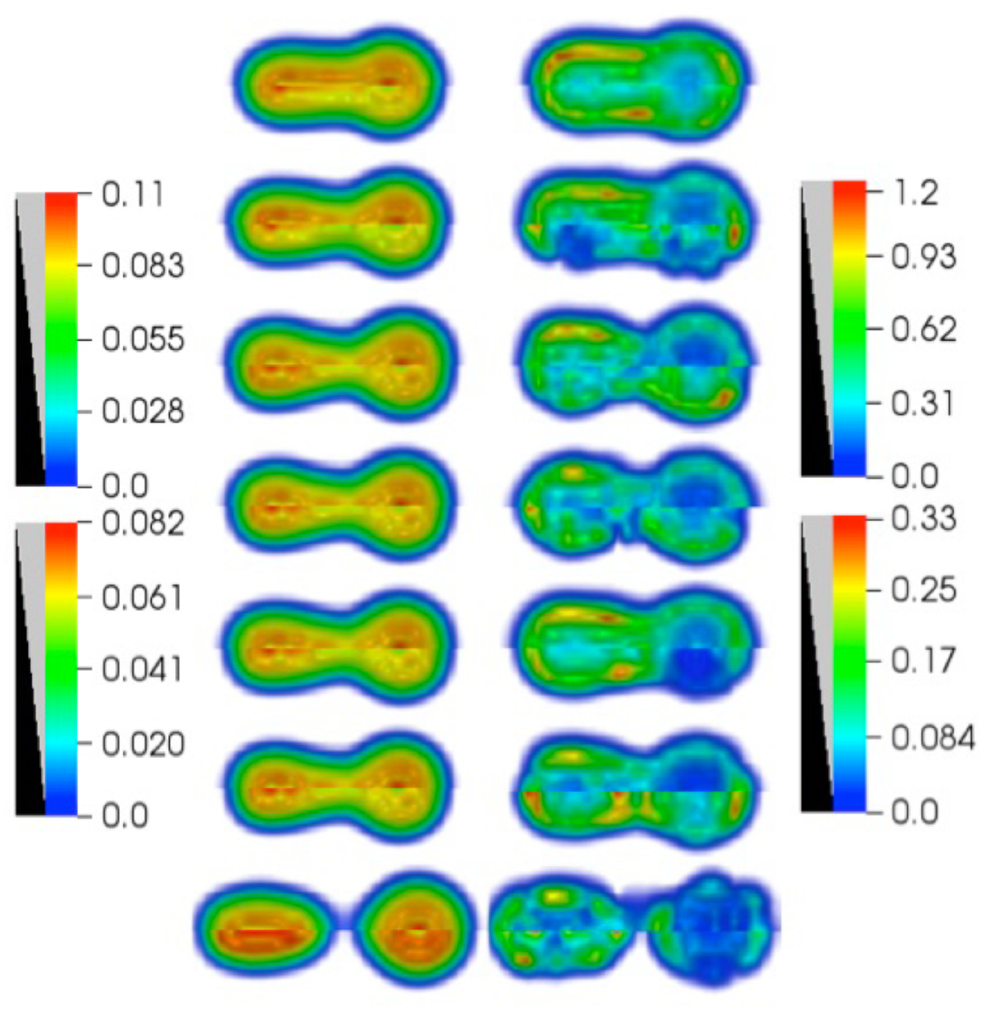