

Abstract
The article aims to determine if a prospective acquisition algorithm can be used to find the ideal set of free-breathing phases for fast-helical model-based 4D-CT. A retrospective five-patient dataset that consisted of 25 repeated free breathing CT scans per patient was used. The sum of the square root amplitude difference between all the breathing phases was defined as an objective function to determine the optimality of sets of breathing phases. The objective function was intended to determine if a specific set of breathing phases would yield a motion model that could accurately predict the motion in all 25 CT scans. Voxel specific motion models were calculated using all combinations of N scans from 25 breathing trajectories, (3 ⩽ N ⩽ 25), and the minimum number of scans required to absolutely characterize the motion model was analyzed. This analysis suggests that the number of scans could potentially be reduced to as few as five scans. When the objective function was large, the resulting motion model provided an excellent approximation to the motion model created using all 25 scans.
Export citation and abstract BibTeX RIS
Introduction
Respiration-induced motion is a considerable source of uncertainty in radiotherapy treatment planning (Keall et al 2006, Kyriakou and McKenzie 2012), and has the potential to lead to substantial dose delivery errors if not properly accounted for (Bortfeld et al 2004). Respiratory-gated 4D computed tomography (4D-CT) offers spatial and temporal information on tumor motion and has become indispensable for the highly conformal treatment of lung tumors (Keall et al 2006). Despite revolutionizing high-dose conformal treatment of lung cancer, conventional 4D-CT methods suffer from image artifacts that can distort structures of interest (Wang et al 2013) and inaccurately characterize breathing motion (Chen et al 2004, Watkins et al 2010), due to the inability to account for irregular breathing.
Current commercial clinical 4D-CT images are typically acquired using either low-pitch helical (Ford et al 2003) or ciné acquisition sequences (Pan 2005, Langner and Keall 2008). Scans are combined with simultaneous breathing surrogate measurements to retrospectively group acquired projections (helical protocols) or images (cine protocols) according to breathing phase, using either amplitude-based or phase-based sorting (Lu et al 2006, Wink et al 2006, Abdelnour et al 2007, Santoro et al 2009). These techniques perform well under conditions of regular breathing with a consistent breathing depth, but image artifacts arise under conditions of irregular breathing (Chen et al 2004), leading to systematic errors in tumor volume and center of mass measurements (Sarker et al 2010). Radiation dose delivered to the patient from a 4D-CT has been reported to be in the range of 4–10 (Matsuzaki et al 2013) times higher than a conventional CT, and although clinical implications may be minimal compared to therapeutic doses, efforts should be made to reduce dose when possible, especially for younger patients.
We recently published a novel 4D-CT technique that employs fast helical CT acquisition, eliminates motion-induced sorting artifacts, and offers potential for dose reduction (Thomas et al 2014). The helical CT scans are acquired with a simultaneous breathing surrogate measurement. The helical CT images were deformably registered to measure the voxel-to-voxel tissue motion and a motion model used to model the voxel motion trajectories as a function of breathing amplitude and rate. In each case, 25 low-dose CT scans were acquired with no breathing gating. We showed that 25 scans acquired at arbitrary breathing phases were more than adequate to sample the breathing cycle over the entire lung, with a mean motion error of 1.3 ± 0.5 mm. Mean motion error was evaluated using a 'leave-one-out' procedure, whereby each scan was left out of the final model fitting in turn, and the tissue locations for that scan were predicted using the model generated without that individual scan. This was compared against the deformably registered tissue locations, allowing a model prediction error to be calculated for each voxel of each scan, and an overall mean value of error to be calculated.
As the scans were acquired at arbitrary breathing phases, invariably some of the CT scans were acquired with nearly the same breathing phases. In a clinical scenario, this would cause acquisition of redundant imaging data, leading to unnecessary patient irradiation. Therefore, we elected to determine if there were a set of breathing phases (i.e. a specific set of breathing signals acquired during scanning) that would provide a motion model that was equivalent to the model developed with the 25 scans and if there was an objective function that could mathematically determine such a combination. While this would not be sufficient to create a prospective CT protocol, as this would require a real-time estimate of the entire breathing phase for the upcoming CT scan, not only the starting phase (Low et al 2005), the work presented here is a necessary pre-requisite for creating such a protocol.
Methods
Under an IRB-approved protocol, five patients were imaged using a 64 slice CT scanner (Siemens Definition Flash). 25 successive low dose scans were performed in alternating directions, under free breathing conditions. Total imaging time ranged from 120 to 160 s, delivering approximately equivalent dose to a conventional low-pitch-helical 4D-CT protocol. Each CT scan was acquired under free-breathing, and an abdominal bellows system (Philips Medical Systems) was used to provide a breathing cycle surrogate. For each patient, the first acquired image was arbitrarily chosen as the reference image. This image was segmented using a region-growing tool in a commercial software package (MIM version 5.6, MIM Software, Cleveland, OH) to isolate the lungs and main-stem bronchi. Deformable image registration (DIR) was implemented on the segmented lung images using an open source software package, 'Elastix'. A B-spline registration algorithm (Werner et al 2010) was used to register the reference image to the subsequent 24 segmented images (the target images). Accurate registration of the shear motion between the lungs and chest wall was achieved by implementing a linear combination of multiple B-spline registrations and ensuring that tissue displacement was continuous in the direction normal to the sliding interfaces, using the lung contour to define the interface (Delmon et al 2013).
The 5D breathing motion model proposed by Low et al (2005) was implemented using fast helical CT data and analysis as described in detail in by Thomas et al (2014). '5D' refers to three spatial dimensions, volume and flow. The registered voxel locations were used to determine the motion model parameters for each voxel, which related tissue motion, calculated from the deformable image registration, to breathing amplitude and rate as measured with a breathing surrogate. In the original work (Low et al 2005) the breathing amplitude and rate were described by the tidal volume and airflow, respectively. These were acquired by normalizing a real-time breathing surrogate measurement consisting of an expandable cylindrical bellows wrapped around the abdomen. The internal air pressure in the sealed bellows varied according to breathing amplitude and was found earlier to be linearly proportional to tidal volume (Werner et al 2010).
Figure 1 describes the workflow of the technique. Low et al (2005, 2013) showed that the deformation a piece of lung tissue undergoes during quiet respiration relative to its position at zero breathing amplitude and rate can be described by a linear approximation in breathing amplitude (v) and rate (f), where v and f are selected as symbols because of the original use of tidal volume and airflow;

where  and
and  related the deformation of the tissue position
  to the breathing amplitude and rate. The position of the tissue at zero amplitude and rate was
  . The parameters
  and
and  were responsible for accounting for motion due to breathing depth and hysteresis, respectively. Time was implicitly considered in the time dependence of the breathing depth and rate.
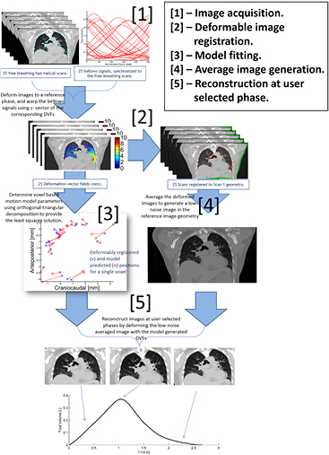
Figure 1. Flow chart describing the motion-model based 4D-CT acquisition and analysis technique. 25 free-breathing fast helical scans are acquired at the same time as surrogate bellows breathing signal. Images are registered to the first scan geometry using B-spline deformable image registration, and the relation between deformation vectors and bellows signals used to generate a motion model.
Download figure:
Standard image High-resolution imageThe motion model parameters were individually determined for each reference image voxel using all N = 25 scans and corresponding breathing phases. For each voxel i, in addition to the reference voxel positions  , there were N − 1 values
  =
= ,
,  ...
...  corresponding to the voxel location in the N different breathing phases, calculated from the deformation vectors. For each reference voxel, there were also the N measured values of breathing amplitude v and rate f at which the voxels were scanned. Equation (1) was solved using a least squares solver applied to each reference voxel i to determine a single set of model parameters
  , and
, and  that described the voxel's free-breathing motion. This process was performed independently in all three directions of the deformation vector field. Solving for the model parameters in all three dimensions in a single coronal slice (512 × 512 voxels, i.e iN = 262 144) for 25 scans (N = 25) using Matlab's (version R2013a; Mathworks, Natick, MA) 'mldivide' function, this process took approximately 10 s (performed with an Intel® i7 PC running at 3.60 GHz). Equation (1) could have been solved for all voxels within the image space, but as the model was to be solved for a large variation of subsets of breathing phases, a single coronal slice was selected to limit the computational time and memory required to calculate the least squares solution.
The model parameters were generated for the central coronal slice using all 25 of the scans. The motion model precision was computed by comparing the motion model predicted tissue positions for a model based on a subset of scans compared to the model computed using all 25 scans. Because we wanted to study motion model precision as a function of the number and selection of breathing phases, the above process was repeated for m phases (where  ), for all combinations of m phases out of the 25 acquired phases. We assumed that the maximum number of scans required to generate a precise motion model was less than or equal to 15, so to limit the number of required computations, only the first 15 scans were considered, although the reference model remained the one calculated using all 25 scans. Rather than compare the motion model for each of the 1 × 1 mm2 coronal voxels, a 10 × 10 subsample was selected for analysis. This also greatly reduced the number of computations.
The goal of this work was to determine if an objective function could be defined that would indicate breathing phases that would yield precision motion models. We used the technique described by Ruan et al (2015) to define the objective function. By calculating the spread of breathing phases in the subset of scans, the independence or redundancy of the amplitude information in that subset could be determined that can eventually lead to a prospective scanning algorithm. The objective function here was calculated from the sum of the square root difference of the breathing phases for the individual axial slice locations of the fast helical scans; by maximizing this function the maximal variation in the motion profile will be achieved.
Results
Figure 2 shows an example of the model residual across the 25 sampled breathing trajectories, for an example voxel in the lower right lung and for the entire image plane. Measured tissue deformations in the craniocaudal (CC) direction are plotted against (a) volume (L) and flow (L/s), and (b) against ante-posterior (AP) motion. In this case, the bellows voltage and rate were transformed to volume and flow by correlating bellows voltage to the lung air content. In (a) and (b) model predicted voxel locations are shown in comparison with voxel location determined directly from the deformable registration. The mean model error across the central coronal slice in is shown in (c), with a mean value of 0.6 ± 0.4 mm.

Figure 2. Measured deformations from the deformable image registration (x) versus model-predicted deformations (o) for an example voxel in the lower right lung of patient #1. The image shown is the reference free-breathing image. (a) Shows the CC motion plotted against volume and flow. (b) Shows CC deformation plotted against AP deformation, showing hysteresis. (c) Color map shows the motion model residual (difference between deformably registered tissue locations and model predicted tissue locations) across both lungs, overlaid on the reference image, with a mean value of  = 0.6 ± 0.4 mm. The reference voxel location of the points shown in (a) and (b) is indicated in the image (circle in the lower right lung).
Download figure:
Standard image High-resolution imageFigure 3 examines the effect of the selection of phases on the resulting motion model. Because of the form of the motion model in equation (1), the motion of a piece of tissue is constrained to lie in a plane with respect to breathing amplitude and rate. This 2D plane is illustrated in figure 3(a) for an example voxel, and for the model calculated using n = N = 25 scans. Scans included in the model calculation are shown in filled circles, and the model predicted locations of the voxels are shown in open circles. Figure 3(a) shows that when n = N = 25, the motion is well modelled, with a mean model residual (the mean difference between measured and model predicted voxel locations) equal to  = 0.6 mm. Figure 3(b) shows the equivalent 2D plane described by the motion model when n = 3, with three well spread breathing phases used to calculate the model parameters. The model parameters were similar to those when n = N = 25, and the resulting plane predicted all 25 voxel locations well, giving a model residual
  = 0.7 mm. Figure 3(c) shows the model result when the phases are closer in phase. The model prediction was worse than the case shown in figure 3(b), with mean model residuals of
  = 0.9 mm. The worst model (figure 3(d) was when two phases were near exhalation (minimum lung volume) and one at mid-exhalation, providing incomplete information on how the lung moved during inhalation. Note the difference in scale on the craniocaudal position axis in figure 3(d). Voxel locations at peak inhalation were poorly extrapolated from these three phases, giving
  = 82.7 mm.

Figure 3. Left column: the 2D plane described by the motion model illustrated for an example voxel in the lower right lung of patient 1. The 25 voxel locations in the CC direction are shown with black x's. Scans included in the model calculation (equation (1)) are shown in filled circles (•), and the model predicted locations of the voxels are shown in open circles (o). Figure (a) shows the results when all scans are used to calculate the model parameters; n = 25. (b)–(d), n = 3, with varying phases included in the three scans, giving increasing model residual for more similar phases. Middle column: color-maps show the mean error per voxel for the corresponding error maps for all voxels within the lungs—note different scale in (d). Right column: the breaths corresponding to each of the error maps.
Download figure:
Standard image High-resolution imageFigure 3 also shows the mean motion model error for the central coronal slice for the models shows in figures 3(a)–(c) (note the scale difference in (d)), ranging from (a) 0.6 ± 0.2 mm (N = 25), (b) 0.7 ± 0.4 mm (n = 3), (c) 0.9 ± 0.8 mm (n = 3), (d) 80 ± 60 mm (n = 3), as well the breathing trajectories associated with each of these subsets. Regions where two of the phases overlapped lead to increased error, due to insufficient motion data being acquired.
The objective function (M) described by Ruan et al (2015) using p = 0.5 was used to evaluate the spread of each subset of breathing trajectories. Figure 4 shows how the value of M correlated with the mean motion model residual ( ) for the subsets
  . For increasing values of n the average motion model accuracy improved, and the variation between specific values of k (i.e. the individual trajectories used to calculate the motion model) were reduced. The minimum mean error achieved for n = 3 was 0.7 ± 0.3 mm, 0.1 mm greater than that the minimum achievable model error. However, the variation in model residual was large, and no correlation with M was observed for n < 5. To determine the correlation of M with
  the variation (mean and standard deviation) of
  for the breathing trajectories corresponding to the maximum 25% of M was calculated, as shown in figure 4(g).
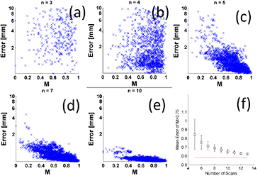
Figure 4. (a)–(f) Variation in the spread of breathing trajectories M with corresponding motion model error for scan subsets of  (log scale on the y-axis limited from 0.1 to 10 mm). Although permutations which correspond to low error exist for all n, and a significant rank correlation between M and error could be found for n = 4, no useful correlation is observed for n < 5. (g) Shows the mean value of error for M > 0.75 in each case (n < 5 not shown). The average error decreases with increasing number of scans n.
Download figure:
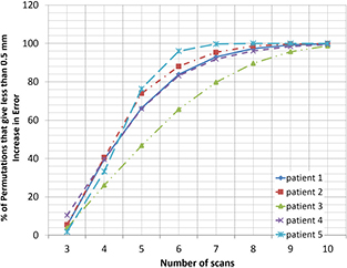
Standard image High-resolution imageFigure 5 shows the percentage of subsets for 5 patients that are able to predict motion to within 0.5 mm of the minimum error possible, showing that 10 scans were sufficient to give the required accuracy, irrespective of the specific breathing trajectories scanned, and the level of breathing irregularity observed.
Figure 5. Variation in the number of breathing trajectories (n) required to give less than 0.5 mm increase in mean model error compared to N = 25. For all patients, all permutations of 10 scans give within 0.5 mm of minimum error.
Download figure:
Standard image High-resolution image
A feature of the comparison between M and the residual error for n  5 was that the greatest values of M guaranteed the lowest values of
  . This implied that for n
  5, there existed a set of phases such that if a large value of M could be prospectively programmed, a small residual model error
  would be guaranteed.
Discussion
The results presented here indicated that prospective gating of free-breathing CT scans could significantly reduce the number of scans required to accurately predict the motion of lung tissue for the fast helical-CT model-based 4D-CT protocol. By monitoring and accurately predicting breathing phases, the acquisition of redundant data could be avoided, reducing both dose delivered to a patient and the time and computation required to produce an artifact free CT at user-specified breathing phases.
By using the results from the objective function to analyze the spread of breathing phases, further improvements to the protocol are possible. The analysis presented in figure 4 suggests that the number of scans could potentially be reduced to as few as five scans if the breathing trace could be predicted with sufficient accuracy to employ prospective CT scan gating. To acquire five scans that would maximize the objective function, a breathing prediction algorithm would be required to select the starting point of the CT scan ('X-Ray On' time) and to accurately predict breathing 1–2 s in advance. Prediction time-steps for a prospectively gated scan would also need to take into account for system latency. White et al (2011) investigated the use of an autoregressive moving average model to predict the breathing trajectories of 47 patients with a conservative 95% confidence criteria giving a maximum prediction time step of 0.3 s. This is too short a time step to predict an exact breathing phases during 1–2 s scans, however the data in figure 4 shows that a range of breathing phases, characterized by M ⩾ 0.75, provide acceptable accuracy, and that additional breathing trajectories might not be required if a 0.3 s prediction time-step were achievable. This could be analyzed in advance of CT scanning by collection of training breathing data. The average error corresponding to M ⩾ 0.75 decreased with n, and the results shown in figure 4 could be used to determine the number of scans required based on a specific patients breathing irregularity.
Conclusions
A fast helical CT model based 4D-CT technique offers potential for improved free breathing imaging while reducing imaging dose. The ideal set of respiratory trajectories required to accurately predict motion using breathing model will depend on the individual motion characteristics of a patient. Application of a simple breathing analysis can predict the minimum number of trajectories required to predict motion to within a given tolerance.