
Abstract
Amplitude modulation of electrostatic Langmuir waves in a quantum electron–hole semiconductor plasma is considered in the quantum magnetohydrodynamic regime. The important ingredients of this study are the inclusion of the particle degeneracy pressure, exchange-correlation potential, and the quantum diffraction effects via the Bohm potential. A nonlinear Schrödinger equation (NLSE) is developed for the evolution of the amplitude of the electrostatic wave by employing the standard reductive perturbation technique. The dynamics of the wave in the slow space-time scales is governed by the NLSE. Typical values of the parameters for GaAs, GaSb, and GaN semiconductors are considered in analyzing the nonlinear dispersion of the electrostatic wave. Detail analysis of the nature of the modulation, here modulation instability, in the long-wavelength regime is presented. For some parameter ranges of the semiconductor plasmas, and at the long-wavelength regime, it is found that the electrostatic wave is modulationally unstable. Effects of the exchange-correlation potential and the Bohm potential are also studied. It is found that the exchange-correlation potential has profound effects compared to the Bohm potential in the amplitude modulation of the electrostatic wave.
Export citation and abstract BibTeX RIS
1. Introduction
Quantum plasma [1–4] has received considerable attention during the past few years because of inevitable applications in emerging miniaturization techniques. A quantum plasma is characterized as a degenerate cold ionized matter. Due to inter-fermion distances much lower than the characteristic de Broglie thermal wavelength in a quantum plasma and the domination of the Pauli exclusion rule, many quantum effects such as electron-tunneling, degeneracy pressure, and Landau quantization may occur [5, 6]. Recent studies based on the quantum hydrodynamics (QHD) model reveal outstanding differences in nonlinear features of quantum plasmas from that of ordinary ones [7–10]. The QHD model is a useful approximation to study the short-scale collective phenomena, such as waves, instabilities, and nonlinear structures in dense plasmas [11, 12]. The QHD model generalizes the usual fluid model with the inclusion of the statistical degeneracy pressure and quantum diffraction (also known as the Bohm potential) terms. The validity of the QHD model is limited to those systems that are large compared to the Fermi lengths of the species in the system.
A possible application of quantum plasma occurs in some astrophysical objects under extreme conditions of temperature and density, such as white dwarf stars, where the density is some ten order of magnitudes larger than that of ordinary solids [13, 14]. Because of such large densities, a white dwarf can be as hot as a fusion plasma, but still behave quantum mechanically. Another possible application of quantum plasmas arises from semiconductor physics [15–18]. Even though the electron density in semiconductors is much lower than in metals, the great degree of miniaturization of todayʼs electronic components is such that the de Broglie wavelength of the charge carriers can be comparable to the spatial variation of the doping profiles. Hence, typical quantum mechanical effects, such as tunneling, are expected to play a central role in the behavior of electronic components to be constructed in the coming years. The study of quantum plasma becomes important when the de Broglie wavelength associated with the charged particles becomes of the order or greater than the inter-particle distance of the system and the plasma behaves like a Fermi gas, and quantum mechanical effects play a significant role in the dynamics. When electrons in the valence band of a semiconductor are excited to the conduction band by absorbing energy, leaving behind vacant electron states called holes, then this system can be considered as a plasma medium because it may satisfy the plasma conditions. For modern device physics experiments with quantum wells, quantum wires, and quantum dots, the collective linear and nonlinear behaviors of waves and instabilities via the dynamics of electrons and holes in the semiconductor are of crucial importance. There are three important quantum mechanical effects that may influence and enhance the collective effects of the semiconductor plasma, and these are the particle degenerate pressure [19], exchange-correlation force [20], and the tunneling of electrons and holes through the Bohm potential [21]. It has recently been found that these effects play important roles in the properties of the acoustic topological solitons, which is obtained from the solution of the Korteweg-de Vries (KdV) equation [22]. It is expected that these quantum mechanical effects may also play important roles in the amplitude modulation of electrostatic waves in these electron–hole semiconductor plasmas. Recent experimental observations of electrostatic solitons in a number of materials and semiconductors, such as Al2O3 [23–26], Si [23, 27], sapphire [28], MgO [23, 29], SiO2[23], and GaAs [30], inspired theoreticians to study and investigate the properties of solitons, particularly the topological solitons as recently studied by Moslem et al [22]. Moslem et al [22] have carried out the study on the acoustic solitary pulses in quantum semiconductor plasmas (GaAs, GaSb, GaN, and InP). They have derived a KdV equation for the propagation of the acoustic solitary waves in the electron–hole semiconductor plasmas. They have reported properties of solitary pulses in such semiconductor plasmas by including the degenerate particle pressure, exchange-correlation effect, and the diffraction effect via the Bohm potential in their analysis. They have found two branches of the electrostatic waves: the Langmuir branch and the acoustic branch. In the lower-frequency branch of the dispersion, it is found in that investigation that a strong localization of acoustic pulses occurs in the semiconductor plasma. Their study reveals that the features of the nonlinear acoustic waves in each semiconductor are different depending upon the typical plasma parameters. In their study, they have not considered the amplitude modulation of the electrostatic waves (the acoustic wave and the Langmuir wave) and a possible modulation instability. Actually, the KdV framework is unable to describe such a possibility. On the other hand, recently, Wang and Lü [31] have studied the modulational instability of the electrostatic acoustic wave mode in quantum electron-hole semiconductor plasmas incorporating collisions among the charge carriers. They have shown that the degenerate pressure has a significant influence on the modulational instablity. It has been shown that the solitary waves in the semiconductor plasmas are damped with time and the damping rate is proportional to the collision. It has been further demonstrated that for long wavelength perturbation, there is a transition of the acoustic mode from a modulationally unstable to a modulationally stable wave.
In our present study, we have derived a nonlinear Schrödinger equation (NLSE) for the Langmuir branch of the electrostatic dispersion relation and have studied in detail the characteristic features of the amplitude modulation and the possibility of modulation instability. We apply the standard reductive perturbation technique [32] to derive the NLSE for the propagation of the nonlinear electrostatic wave in the semiconductor plasma as an envelope soliton. We also discuss the possible modulation instability of the electrostatic wave amplitude and carry out some parameter studies for different semiconductors on the envelope soliton.
The paper is organized as follows. Section 2 describes the hydrodynamical model of the quantum electron–hole semiconductor plasma and presents the set of highly nonlinear equations for the evolution of the large-amplitude electrostatic wave pulse. In this section, an NLSE is derived by applying the reductive perturbation technique. A nonlinear dispersion relation and hence an expression for the growth rate of the modulation instability of the electrostatic wave is derived in this section. Results are discussed in section 3 along with graphical representation. Finally, section 4 concludes the paper.
2. The Mathematical Model
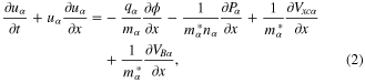
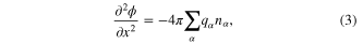
We consider the propagation of a large-amplitude nonlinear electrostatic wave in a two-component quantum plasma composed of electrons and holes. The nonlinear dynamics of such disturbances are governed by the following set of fluid equations [22]:

where  (for electrons) and
  (for holes),
  is the charge,
  is the effective mass,
  and
and  are, respectively, the particle number density and fluid velocity of particle species α;
  for electrons and
  for holes, and e is the magnitude of the electronic charge; ϕ is the electrostatic potential. The second term in the right-hand side of equation (2) is due to the non-relativistic degenerate particle pressure
  and is given by [19]:
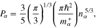
where  , h is the Planck constant. The third term in the right-hand side of equation (2) is due to the exchange-correlation potential
  of the plasma particles and is given by [20]:
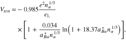
where  is the linear dielectric constant of the semiconductor, and
  is defined as
  . The last term of the right-hand side of equation (2) is due to the tunneling effect of the plasma particles via the Bohm potential [21]:
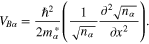
The variables appearing in equations (1)–(3) are to be appropriately normalized. Accordingly, we normalize as follows:  ,
,  is the equilibrium particle number density;
  , where
 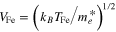 is the electron Fermi velocity,
  is the electron Fermi temperature and is obtained from the relation
  , where
  is the electron Fermi energy and is given by [33]:
  ,
,  is the band gap between the valence band and the conduction band of the semiconductor and
  is the bulk plasma temperature,
  is the Boltzmann constant;
  ;
;  ,
, 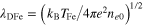 is the Fermi electron Debye length;
  ,
, 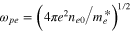 is the electron plasma frequency. It is to be mentioned here that the equilibrium particle number densities of the electron and hole plasma species of the electron–hole plasma are equal:
  . After these normalizations, the set of equations, equations (1)–(3), take the following forms:

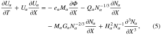
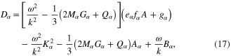
where  ,
,
and 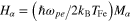 . It is to be mentioned here that the second, third, and fourth terms of the right-hand side of equation (5) are, respectively, due to the non relativistic pressure of the degenerate electrons and holes, electron and hole exchange-correlation force, and quantum recoil force associated with the Bohm potential.
Now, we apply the standard reductive perturbation technique [32], with the following stretched coordinates:  and
and  , where λ is a constant and will be determined later from the compatibility condition of the reductive perturbation analysis and
  is a small positive quantity less than 1, which is the perturbation parameter. Expanding the dependent variables
  ,
,  , and Φ as

where ω and k are the angular frequency and the wavenumber of the carrier electrostatic wave. The quantities  ,
,  , and
, and  are the
  th harmonic of the
  th order slowly varying field variables
  ,
,  , and Φ, respectively. If we substitute the previous expansions for the field variables in the set of equations given by equations (4)–(6), we can easily obtain the
  th harmonic of the
  th order reduced equations. We omit listing the reduced equations here, as they are very lengthy and will not be much use to most of the readers.
2.1. Linear dispersion relation for the electrostatic wave
If we consider the first harmonic of the first-order quantities ( and
and  ) in the reduced equations, the following linear dispersion relation of the electrostatic wave is easily obtained:
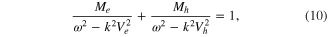
where 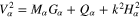 . Similarly, from the first harmonic of the second-order quantities (
 and
and  ), and using equation (10), we obtain the following compatibility condition, which gives the group velocity λ:

where 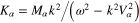 .
.
The detail analysis of the linear dispersion relation given by equation (10) is given earlier by Moslem et al [22] and hence we do not discuss this further. It should be mentioned here that there are two branches of the linear dispersion relation: one for a comparatively higher frequency ( ), called the Langmuir wave mode, and the other for a lower-frequency wave (
 ), called the acoustic wave mode. Moslem et al [22] have considered the lower-frequency branch, the acoustic wave mode, in their study of the topological soliton through the KdV equation. Similarly, Wang and Lü [31] have also considered only the lower frequency branch, the electrostatic acoustic wave mode, for the study of the modulational instability of the electrostatic wave in quantum electron-hole semiconductor plasmas. However, we consider in our analysis the higher-frequency branch, the Langmuir wave mode, for the nonlinear amplitude modulation. Because of the possible linear Landau damping, we consider only the long wavelength perturbation (small carrier wavenumber,
  ) for the propagating Langmuir wave mode. For simplicity of analysis of our results, we have neglected the collision among the charge carriers in the electron-hole plasma.
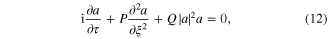
2.2. The NLSE and its solution
Here, we do not go into the detail derivation of the NLSE, but only state briefly the procedure. From the  part of the second-order (
 ) reduced equations, the second-order harmonic mode
  of the carrier wave is obtained in terms of
  , where
  is the first-order mode, obtained in deriving the linear dispersion relation, equation (10). The mode
  comes from the nonlinear self-interaction. Similarly, from the
  part of the third-order (
 ) reduced equations, the zeroth harmonic mode
  is obtained in terms of
  . Its expression cannot be obtained from the second-order equations. Finally, substituting the expressions for
  and
and  into the
  component of the third-order (
 ) part of the reduced equations, we finally obtain the following NLSE:
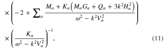
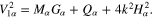
where  and
and
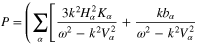
and
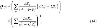
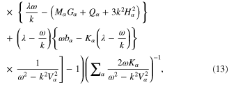
In equations (13) and (14), the quantities  ,
,  , and
, and  are given by

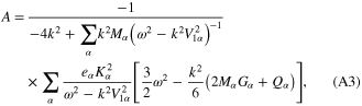
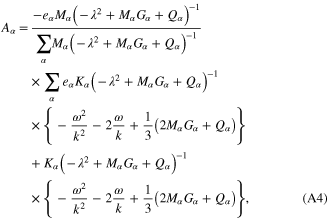
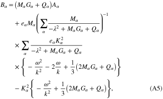
and the quantity  is defined earlier. The parameters
  ,
,  , A,
, A,  , and
, and  appearing in equations (16) and (17) are given in appendix.
The coefficients P and Q appearing in the NLSE, given by equation (12), are known as the dispersion coefficient and nonlinear coefficient, respectively. The signs of P and Q determine whether the slowly varying wave amplitude is stable or not. If the signs of P and Q are such that  , the wave amplitude is modulationally stable and the corresponding solution of the NLSE is called a dark soliton [34]. On the other hand, if
  , then the wave amplitude may be modulationally unstable, and the solution of the NLSE in this case is called a bright soliton [34]. We are particularly interested in the bright soliton in this paper; for this, we do some detail parameter studies on the behavior of the bright soliton, which is discussed in section 3.
Applying the standard technique, the following solution of the NLSE, equation (12), is easily obtained in the case of  :
:
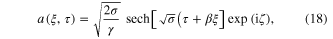
where  is the modulation phase and
  and
and  are, respectively, the wavenumber and frequency of the modulation,
 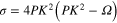 ,
,  and
and  . The peak pulse power is defined as
  and the pulse width is defined as
  .
.
2.3. Nonlinear dispersion relation for the amplitude modulation of electrostatic Langmuir waves
We now analyze the stability and possible modulational instability of the slowly varying electrostatic wave (the Langmuir wave) in the degenerate quantum electron–hole semiconductor plasma. Instead of a static solution, we consider the dynamic solution of the NLSE.
Accordingly, we separate the amplitude a into two parts:
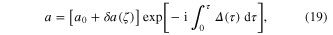
where a0 is the constant (real) amplitude of the pump carrier wave  ,
,  is the small-amplitude perturbation, and Δ is a possible nonlinear frequency shift. After substituting equation (19) into the NLSE, equation (12), and following standard technique [35], the following nonlinear dispersion relation for the amplitude modulation of the electrostatic wave in the e–p plasma is obtained:
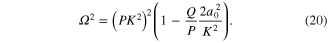
For the parameters satisfying  , we see from equation (20) that there is a possibility of modulational instability. This happens if
  . In this situation,
  . Then, assuming
  , we find from equation (20):
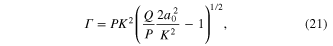
as the growth rate of the modulational instability of the nonlinear electrostatic wave, where expressions for P and Q are given by equations (13) and (14), respectively.
3. Results and discussions
In this section we analyze the properties of amplitude-modulated solitons of Langmuir waves in the electron–hole plasma. For the numerical appreciation of our results, we have selected three types of semiconductors: GaAs, GaSb, and GaN. The typical parameters of these semiconductors at temperature  K [6, 36, 37] are listed in table 1.
Table 1. Typical plasma parameters.
| GaAs | GaSb | GaN | |
|---|---|---|---|

|
 cm−3 cm−3 |
 cm−3 cm−3 |

|
 cm−3 cm−3 |
|||

|

|

|

|

|

|

|

|

|
12.80 | 15.69 | 11.30 |

|
1.43 eV | 0.78 eV | 3.40 eV |
Figure 1 shows the variation of the product PQ, of the dispersive coefficient P, and the nonlinear coefficient Q with respect to the carrier wavenumber k for three different types of semiconductors: GaAs, GaSb, and GaN, keeping all the nonlinear terms, viz, the term due to the degenerate particle pressure, determined by the coefficient  ; the term due to the exchange-correlation potential, determined by the coefficient
  ; and the term due to the Bohm potential, determined by the coefficient
  in the particle momentum balance equation. In the aforementioned, α indicates particle species electron (e) and hole (h). The solid, dotted, and dashed curves are, respectively, for the semiconductors GaAs, GaSb, and GaN. We see from this figure that for all three semiconductors, the product PQ is positive for the long wavelength perturbation (
 ), indicating that the electrostatic wave mode (the Langmuir wave) may be modulationally unstable. We observe from figure 1 that for the whole range of the normalized wavenumber, k = 0-0.5, the nonlinear Langmuir wave is modulationally unstable, which is in contrast to the case of the electrostatic acoustic wave studied by Wang and Lü [31], where the wave is modulationally unstable for the range of the wavenumber k = 0-0.4 and then the wave becomes modulationally stable for the wavenumber k > 0.4.
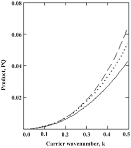
Figure 1. Variation of the product PQ versus the carrier wavenumber k. The solid, dotted, and dashed curves are for GaAs, GaSb, and GaN, respectively. In this figure, effects of particle degenerate pressure, particle exchange-correlation potential, and Bohm potential are included.
Download figure:
Standard image High-resolution imageFigure 2 shows the amplitude of the bright soliton  with respect to the relative argument
  , for the three types of semiconductors, keeping all three terms due to the degenerate particle pressure, the exchange-correlation potential, and the Bohm potential in the analysis. The solid, dotted, and dashed curves are, respectively, for the semiconductors GaAs, GaSb, and GaN. We observe from this figure that the amplitude of the bright soliton for the case of GaN is tallest while the width is narrowest, and the amplitude for GaAs is the lowest while its width is the widest.
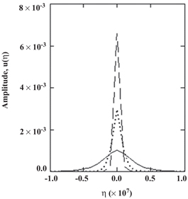
Figure 2. Soliton amplitude  , where
  , τ and ξ have been defined earlier. The solid, dotted, and dashed curves are for GaAs, GaSb, and GaN, respectively. In this figure, effect of the degenerate particle pressure, particle exchange-correlation potential, and the Bohm potential are included.
Download figure:
Standard image High-resolution imageFigure 3 shows the amplitude of the bright soliton  with respect to the relative argument η for the case of the GaN semiconductor, taking the equilibrium electron number density
  as a parameter while keeping all three terms due to the degenerate particle pressure, the exchange-correlation potential, and the Bohm potential in the analysis. The solid, dotted, and dashed curves are, respectively, for
  cm−3,
cm−3,  cm−3, and
  cm−3. We observe from this figure that as the density increases, the amplitude of the bright soliton also increases while its width decreases.
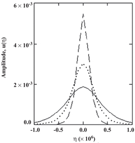
Figure 3. Soliton amplitude  for GaN, taking electron number density
  as a parameter, where
  τ and ξ have been defined earlier. The solid, dotted, and dashed curves are for
  cm−3,
cm−3,  cm−3, and
  cm−3 respectively. Other parameters are as follows:
  ,
,  , and
, and  . In this figure, effect of the degenerate particle pressure, particle exchange-correlation potential, and the Bohm potential are included.
Download figure:
Standard image High-resolution imageFigure 4 shows the amplitude of the bright soliton  with respect to the relative argument η for the case of the GaN semiconductor. The solid curve is for when all three effects, particle degeneracy pressure, exchange-correlation potential, and the Bohm potential, are included in the momentum balance equations for the species electrons and holes; the dotted curve is for when the Bohm potential is excluded, while the dashed curve is for when the exchange-correlation potential term is excluded. An interesting observation from this figure is that the curve when all three terms are included and the curve when the Bohm potential is excluded coincide each other, indicating that the Bohm potential term is not important in the soliton amplitude. However, from the dashed curve we observe that when the exchange-correlation potential term is excluded, then the amplitude of the bright soliton drastically falls and the width becomes wider, indicating that the exchange-correlation potential term is much more important than the Bohm potential term.
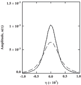
Figure 4. Soliton amplitude  for GaN. The solid curve is for when the effect of particle degenerate pressure, exchange-correlation potential, and Bohm potential all are included; the dotted curve is for when the effect of the Bohm potential is excluded; and the dashed curve is for when the effect of exchange-correlation potential is excluded. Other parameters are as follows:
  ,
,  , and
, and  .
.
Download figure:
Standard image High-resolution imageFigure 5 shows the variation of the modulational instability growth rate Γ with respect to the carrier wavenumber k for the semiconductor GaN, taking electron number density  as a parameter. The solid, dotted, and dashed curves are for
  cm−3,
cm−3,  cm−3, and
  cm−3 respectively. In this figure, effects of particle degeneracy pressure, exchange-correlation potential, and Bohm potential are all included. We observe from this figure that as the equilibrium electron number density increases, the growth rate curves are shifted to the right in the Γ versus k diagram, indicating that scope for the modulation growth rate decreases in terms of the carrier wavenumber k.
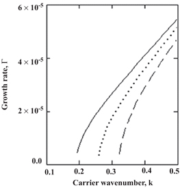
Figure 5. Variation of the modulational instability growth rate Γ with respect to the carrier wavenumber k for the semiconductor GaN, taking electron number density  as a parameter. The solid, dotted, and dashed curves are for
  cm−3,
cm−3,  cm−3, and
  cm−3 respectively. Other parameters are as follows:
  ,
,  , and
, and  . In this figure, effects of particle degeneracy pressure, exchange-correlation potential, and Bohm potential are all included.
Download figure:
Standard image High-resolution imageFigure 6 shows the variation of the modulational instability growth rate Γ with respect to the modulation wavenumber K for the semiconductor GaN, taking electron number density  as a parameter. The solid, dotted, and dashed curves are for
  cm−3,
cm−3,  cm−3, and
  cm−3 respectively. In this figure, effects of particle degeneracy pressure, exchange-correlation potential, and Bohm potential are all included. It is observed from this figure that as the equilibrium electron number density increases, the growth rate of the modulation instability decreases in the comparatively higher modulation wavenumber.
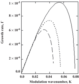
Figure 6. Variation of the modulational instability growth rate Γ with respect to the modulation wavenumber K for the semiconductor GaN, taking electron number density  as a parameter. The solid, dotted, and dashed curves are for
  cm−3,
cm−3,  cm−3, and
  cm−3 respectively. Other parameters are as follows:
  and
and  . In this figure, effects of particle degeneracy pressure, exchange-correlation potential, and Bohm potential are all included.
Download figure:
Standard image High-resolution imageFigure 7 shows the variation of the modulational instability growth rate Γ with respect to the carrier wavenumber k for the semiconductor GaSb. The solid curve is for when the effect of particle degeneracy pressure, exchange-correlation potential, and Bohm potential are all included; the dotted curve is for when the effect of the Bohm potential is excluded; and the dashed curve is for when the effect of exchange-correlation potential is excluded. It is observed from this figure that at the much lower values of the carrier wavenumber there is not much difference in the growth rate of the instability, while as the carrier wavenumber increases, then the effects of the different terms start to show up.

Figure 7. Variation of the modulational instability growth rate Γ with respect to the carrier wavenumber k for the semiconductor GaSb. The solid curve is for when the effect of particle degenerate pressure, exchange-correlation potential, and Bohm potential all are included; the dotted curve is for when the effect of the Bohm potential is excluded; and the dashed curve is for when the effect of exchange-correlation potential is excluded. Other parameters are as follows:  and
and  .
.
Download figure:
Standard image High-resolution imageFinally, figure 8 shows the variation of the modulational instability growth rate Γ with respect to the modulation wavenumber K for the semiconductor GaSb. The solid curve is for when the effect of particle degeneracy pressure, exchange-correlation potential, and Bohm potential are all included; the dotted curve is for when the effect of the Bohm potential is excluded; and the dashed curve is for when the effect of exchange-correlation potential is excluded. This figure shows that the instability growth rate accommodates the drastic effect of the exchange-correlation potential term, while it does not change due to the absence of the Bohm potential term in the momentum balance equation in the model.
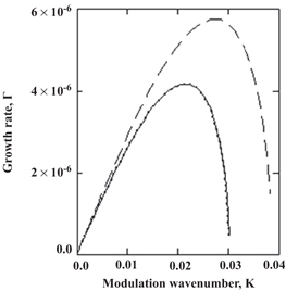
Figure 8. Variation of the modulational instability growth rate Γ with respect to the modulation wavenumber K for the semiconductor GaSb. The solid curve is for when the effect of particle degenerate pressure, exchange-correlation potential, and Bohm potential all are included the dotted curve is for when the effect of the Bohm potential is excluded; and the dashed curve is for when the effect of exchange-correlation potential is excluded. Other parameters are as follows:  and
and  .
.
Download figure:
Standard image High-resolution imageIt should be mentioned here that for a modulationally unstable electrostatic wave, the amplitude gets amplified with time. As the soliton amplitude becomes very large and the perturbation scheme that we adopted breaks down, the soliton explodes or collapses depending on the conservation of energy within the soliton profile. Both these features are of similar nature, but differ by the fact that if the amplitude grows without maintaining the soliton properties, i.e., conservation of energy within its profile, the large amplitude causes explosion of the soliton. The collapsed soliton, on the other hand, may give rise to a large amplitude electrostatic wave. In either case, there is a formation of a narrow wave packet, generating high energy and propagating with high speed, which has the features of soliton radiation [38].
4. Conclusion
We have investigated the nonlinear wave dispersion of an electrostatic Langmuir wave pulse in quantum electron–hole semiconductor plasmas. An NLSE is derived for the slow evolution of the Langmuir wave amplitude. We have discussed the nonlinear dispersions of the wave propagating in the semiconductor plasmas. For three types of semiconductors, viz, GaAs, GaSb, and GaN, for some physically realizable parameter sets, and in the limit of long wavelength perturbations (small carrier wavenumber  ), the electrostatic wave amplitude is unstable. For the case of the modulationally unstable wave, we have investigated in detail the effects of the particle degeneracy pressure, exchange-correlation potential, and the Bohm potential on the amplitude of the bright soliton, and also on the growth rate of the modulation instability of the bright soliton, which is obtained from the solution of the NLSE. We have also studied the growth rate dependencies on the carrier wavenumber k as well as on the modulation wavenumber K. From the numerical results, it is found that the carrier wavenumber, modulation wavenumber, and the type of semiconductor have profound effects on the dispersion properties of the electrostatic wave. Important ingredients introduced in this investigation are the inclusion of the quantum statistical degeneracy pressure, exchange-correlation force, and the quantum diffraction effect via the Bohm potential. It has been found that the exchange-correlation potential has a profound effect, while the Bohm potential has a negligible effect on the nonlinear amplitude modulation of the electrostatic Langmuir wave. In conclusion, we stress that the soliton and its stability investigated in this paper can be associated with electrostatic disturbances that can occur in electron–hole semiconductor plasmas [39].


