Precision spectroscopy of 2S–nP transitions in atomic hydrogen for a new determination of the Rydberg constant and the proton charge radius

Axel Beyer; Lothar Maisenbacher; Ksenia Khabarova; Arthur Matveev; Randolf Pohl; Thomas Udem; Theodor W Hänsch; Nikolai Kolachevsky

doi:10.1088/0031-8949/2015/T165/014030

1. Introduction

Precision spectroscopy of atomic hydrogen, the simplest atomic system, has been one of the key tools for testing fundamental theories of light, matter and their interaction ever since the dawn of modern physics. Starting from the simple empirical formula by Balmer in 1885, that described the numerous distinct absorption and emission lines in the visible spectrum of atomic hydrogen, the theoretical description of the energy levels has been evolving over the last century, revolutionizing our basic understanding of nature not only once. In 1913, Bohr was the first to use the idea of matter waves to explain the discrete spectrum of atomic hydrogen. In his well known planetary model of the atom, he proposed stationary states to be the ones where the orbit circumference matches an integer multiple of the electron de Broglie wave length. Shortly thereafter, the emerging field of quantum mechanics was put on solid grounds by the first wave equation for matter waves formulated by Schrödinger. Solving the stationary Schrödinger equation of an electron bound to an infinitely heavy, point-like proton gives the same simple dependence of the energy levels E_n on the principal quantum number n as predicted by the Bohr theory:

$\begin{eqnarray}&&{E}_{n}=-\frac{{R}_{\infty }}{{n}^{2}}\end{eqnarray} \tag{ 1 }$

where ${R}_{\infty }$ denotes the Rydberg constant. Increasing experimental accuracy and the observation of the fine structure in the hydrogen spectrum, i.e. the fact that the spectral lines in the Balmer series for example consist of doublets rather than single lines, which had not been predicted by the Bohr and Schrödinger theory, triggered the next major step in theory: Dirac reformulated the Schrödinger equation in 1928, including relativistic effects and introducing the electron spin. The Dirac equation withstood two decades of experimental tests, before Lamb and Retherford discovered a discrepancy with the theory in 1947 [1]: 'the results indicate clearly that, contrary to theory [...], the ${2}^{2}{{\rm{S}}}_{1/2}$ state is higher than the ${2}^{2}{{\rm{P}}}_{1/2}$ by about 1000 Mc s⁻¹ [1 GHz].' According to the Dirac theory, these two states with equal principal quantum number $n=2$ and total angular momentum quantum number $j=1/2$ had been expected to be degenerate in energy although their orbital angular momentum quantum numbers are different (S and P). However, this discrepancy had not been caused by shortcomings of quantum theory itself, but rather by the fact that quantum mechanics had not been applied in its most rigorous way, as has been shown later by the pioneers of quantum electrodynamics (QED), Ühling, Bethe, Feynman and others. In particular, the way the quantum vacuum—both electronic and photonic contributions—affects the energy levels in atomic hydrogen had not been accounted for yet. Since then, QED passed every experimental test undertaken in the last 65 years and survived six orders of magnitude in improvement of experimental accuracy. Of course, several discrepancies between QED and experiments have shown up during this time, but all of them could be traced back to either neglected higher order terms in the calculations or underestimated experimental error bars.

2. QED description of the hydrogen atom

The theoretical description in the framework of QED expresses the energy levels in atomic hydrogen as ${R}_{\infty }f(\alpha ,{m}_{{\rm{e}}}/{m}_{p},{r}_{p},...)$ , i.e. as a product of the Rydberg constant ${R}_{\infty }$ and a dimensionless function f that represents the energies in Rydberg units. f is a function of the fine structure constant α, the electron-to-proton mass ratio ${m}_{e}/{m}_{p}$ and the proton root mean square (rms) charge radius r_p, while the Rydberg constant ( ${R}_{\infty }=10\;973\;731.568\;539(55){{\rm{m}}}^{-1}$ [2]) serves as a unit converter from Rydberg units to S.I. units. To be precise, even more parameters enter f, e.g. the ratio of the electron mass to Planck's constant ${m}_{e}/h$ . But at the current level of accuracy, those parameters play a minor role as will be discussed in the next paragraph. Like most QED results, the energy levels can be written as a power series in α:

$\begin{eqnarray}E & = & {R}_{\infty }\left(-\displaystyle \frac{1}{{n}^{2}}+{A}_{20}{\alpha }^{2}+{A}_{30}{\alpha }^{3}+{A}_{31}{\alpha }^{3}{ln}(\alpha )\right.\\ & & +\left.{A}_{40}{\alpha }^{4}+\;\ldots \;+\displaystyle \frac{16{\pi }^{2}{m}_{e}^{2}{c}^{2}{\alpha }^{2}}{3{n}^{3}\;{h}^{2}}\ {\delta }_{l0}{r}_{p}^{2}\right).\end{eqnarray} \tag{ 2 }$

Comparing equations (1) and (2) illustrates a conceptual drawback of the developments sketched in the previous section: not only became our description of nature more complicated over the decades, it also requires an entire set of parameters which can not be calculated from first principles. While for the non-relativistic Bohr and Schrödinger theory—reproduced by the leading order term in equation (2)—only the Rydberg constant was needed as an external input parameter, the full QED description needs additional parameters: higher order terms add corrections to the simple non-relativistic result, such as terms for relativistic recoil, the electron self energy and vacuum polarization. In addition to the quantum numbers describing the particular state of interest, the coefficients A_mn used in these terms also depend on the electron-to-proton mass ratio ${m}_{e}/{m}_{p}$ . A compilation of all known A_mn can be found in [2]. The last term in equation (2) is the leading order finite size correction. This correction arises due to the fact that the proton is not a point-like particle and accounts for the corresponding modifications of the proton's Coulomb potential seen by the electron depending on its particular orbit. These corrections are particularly important for states with a large overlap between electron wave function and the nucleus, i.e. for S-states where the electron is more likely to be found inside the proton. Since the finite size correction only adds a small contribution to the total energy and is entirely limited by the uncertainty of r_p (see e.g. [3]), the other parameters involved in this term can be taken from other experiments with sufficient accuracy. In order to determine the remaining four parameters, a combination of four measured transition frequencies in atomic hydrogen could in principle be used, but due to their higher sensitivity to individual parameters, precision measurements in other branches of physics offer more precise values for some of them: the fine structure constant can be extracted with an uncertainty of 3.7 parts in 10¹⁰ from the measurement of the free electron g-factor [4] and the corresponding QED expression [5]. This value is in agreement and three orders of magnitude more accurate than the value from hydrogen spectroscopy (see [2], equation (88)). Furthermore, mass ratios for particles which can simultaneously be held in a Penning trap can be determined with relative uncertainties on the order of 10⁻¹¹ by comparing their cyclotron frequencies [6]. This way, the electron-to-proton mass ratio has been determined with an uncertainty lower than from equation (2) given the accuracy of the data currently available from hydrogen spectroscopy [7].

3. The proton size puzzle

Following the arguments of the previous section, there are two parameters left to be determined to enable QED calculations competitive with current experimental accuracy: the Rydberg constant and the proton rms charge radius. These parameters can be extracted from a combination of two measured transition frequencies in hydrogen, while the comparison of results obtained from different pairs probes the internal consistency of the corresponding QED calculations.

The 1S–2S transition frequency with its relative uncertainty of a few parts in 10¹⁵ is the most accurately measured transition frequency in atomic hydrogen [8, 9]. Combining this result with each of the other measured transition frequencies listed in Table XI of the CODATA 2010 report [2], one obtains 15 pairs of values for ${R}_{\infty }$ and r_p. Depicted in figure 1(a) are only the values for r_p, since the corresponding plot for ${R}_{\infty }$ does not add much information due to the 96% correlation of the two parameters. A measure for the internal consistency of the values extracted is the Birge ratio R_B, i.e. the square root of the weighted mean quadratic deviation from the data set's weighted mean. For Gaussian distributed data, R_B = 1 with a variance equal to $2/(N-1)$ where N is the number of data points. For the proton charge radii shown in figure 1(a), ${R}_{{\rm{B}}}=0.70(38)$ is compatible with Gaussian scatter of the results. Although this simple approach uses the 1S–2S transition frequency multiple times in the extraction process, its influence on the overall uncertainty of the results is negligible because its relative uncertainty is three orders of magnitude smaller than any of the other transition frequencies involved. The proper way to extract best estimates for the value pair [ ${R}_{\infty }$ , r_p] is to perform a least squares adjustment for the entire data set at once. The corresponding result of ${r}_{p}=0.8764(89)\;\mathrm{fm}$ can be found in 'adjustment #8' in table XXXVIII in the CODATA report [2].

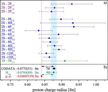
**Figure 1.** (a) The root mean square proton charge radius r_p extracted from precision spectroscopy of atomic hydrogen. Experiments either probe transitions in the radio frequency (violet, historically called Lamb shift measurements) or optical domain (blue from the 2S state, green from the 1S sate). In order to obtain a value pair [ ${R}_{\infty }$ , r_p], each transition frequency needs to be combined with another independent measurement, in the case shown, this is the 1S–2S transition frequency. The radio frequency measurements are much more sensitive to r_p and less sensitive to ${R}_{\infty }$ than the experiments in the optical domain. Therefore significantly lower experimental accuracy and a moderately accurate determination of ${R}_{\infty }$ suffice to extract accurate values of r_p from these measurements. (b) A discrepancy of four combined standard deviations is found, when comparing the hydrogen average value (H_avg) with the value obtained from muonic hydrogen spectroscopy (red diamond). An even larger discrepancy of 7σ is obtained when a selection of electron–proton scattering data is included in the analysis, as has been done in the CODATA adjustment of fundamental constants (black square) [2].
Download figure:
Standard image High-resolution image

**Figure 1.** (a) The root mean square proton charge radius r_p extracted from precision spectroscopy of atomic hydrogen. Experiments either probe transitions in the radio frequency (violet, historically called Lamb shift measurements) or optical domain (blue from the 2S state, green from the 1S sate). In order to obtain a value pair [ ${R}_{\infty }$ , r_p], each transition frequency needs to be combined with another independent measurement, in the case shown, this is the 1S–2S transition frequency. The radio frequency measurements are much more sensitive to r_p and less sensitive to ${R}_{\infty }$ than the experiments in the optical domain. Therefore significantly lower experimental accuracy and a moderately accurate determination of ${R}_{\infty }$ suffice to extract accurate values of r_p from these measurements. (b) A discrepancy of four combined standard deviations is found, when comparing the hydrogen average value (H_avg) with the value obtained from muonic hydrogen spectroscopy (red diamond). An even larger discrepancy of 7σ is obtained when a selection of electron–proton scattering data is included in the analysis, as has been done in the CODATA adjustment of fundamental constants (black square) [2].
Download figure:
Standard image High-resolution image

Historically, r_p has been determined by elastic electron–proton scattering experiments. In the mid 1990s, though, hydrogen spectroscopy experiments and the corresponding theory became accurate enough to extract r_p with an uncertainty of about 1%. The value extracted from hydrogen spectroscopy had been the most precise, until in 2010, laser spectroscopy of muonic hydrogen provided a new value ten times more accurate than any previous determination [10]. Muonic and electronic hydrogen are similar systems regarding their treatment in the framework of QED, but the muon is about 200 times heavier than the electron. Accordingly, the weight of the finite size correction is scaled up by 200² relative to the other contributions in equation (2) when replacing m_e by ${m}_{\mu }$ . In S.I. units, the finite size effect is 200³ times larger in muonic hydrogen, taking into account that another factor of m_e is hidden within the Rydberg constant ${R}_{\infty }=({m}_{e}{\alpha }^{2}c)/2\;h$ . With this enhanced sensitivity, moderate accuracy in the determination of the 2S– $2{{\rm{P}}}_{3/2}$ transition frequency and 5 out of the 12 known digits of the Rydberg constant are sufficient to obtain this impressive accuracy in r_p. Meanwhile, the muonic hydrogen value has been confirmed and improved [11], yielding ${r}_{p}=0.840\;87(39)\;\mathrm{fm}$ , a value about 4% smaller than the values extracted from electronic hydrogen and elastic electron–proton scattering.

A 4% difference may seem small at first glance, but since electronic and muonic hydrogen are so similar in their theoretical description, figure 1(b) reveals a highly unsatisfying situation: the proton charge radius (and the Rydberg constant) extracted from these two systems (H_avg and $\mu -p$ ) are discrepant by four combined standard deviations. An even larger discrepancy of 7σ is found when including a selection of electron–proton scattering data into the analysis as has been done in the 'adjustment #3' in the CODATA report, shown as a black square in figure 1(b). This discrepancy is referred to as 'the proton size puzzle' and although many efforts have been undertaken in the last years, no convincing solution could be found so far. For a detailed discussion of possible ways to resolve the puzzle, we refer to the review [12], while the rest of this text will focus on the electronic hydrogen part.

For the existing hydrogen data set, the longest lever arm on the puzzle can be found in improving measurements of transition frequencies starting from the metastable 2S state. Violet squares in figure 1(a) represent radio frequency measurements of the 2S Lamb shift, i.e. the energy splitting between 2S and 2P states, whereas blue points represent optical measurements in the visible range. Each one of these individual measurements is compatible with the muonic hydrogen value within a few standard deviations, while the discrepancy of 4σ only arises when the data is averaged. On the other hand, to account for the discrepancy, the 1S–2S transition frequency which is used as a corner stone in the extraction would need to be off by 4000 experimental error bars and the value extracted from muonic hydrogen by 100σ. Both experiments have been confirmed and improved recently, making this seem rather improbable. Hence, additional data input for the 2S–nL transitions is highly desirable to gain deeper insight into the apparent discrepancy. In the ideal case, a single experiment would have an uncertainty comparable to the one of the aggregate electronic hydrogen data set or better to exclude possible systematic efffects on the order of the discrepancy to be hidden within the experimental error bars. In addition, the re-measurements of the 1S–3S transition frequency (green triangle) underway in Paris and Garching [14, 15] can strengthen the extraction of the value pair [ ${R}_{\infty }$ , r_p] by providing redundant input complementary to the 1S–2S frequency.

4. The hydrogen 2S–4P transition

4.1. The choice of the transition

There is no easy-to-follow recipe on how to choose a candidate transition to obtain additional input for the electronic hydrogen part of the proton radius puzzle. Each choice has its justification and goes along with a set of compromises a particular experiment has to deal with.

Starting spectroscopy experiments from the 1S ground state offers the advantage of having a large atomic population to start with. The drawback is that short wavelengths are required to drive these transitions. In practice, only two photon transitions with $n=2,3,4$ are addressable with simple means of frequency doubling or sum frequency conversion in commercially available non-linear optical materials [14, 15]. Probing two photon transitions in general also provides the benefit of small natural line widths, while this advantage comes at the price of high excitation light powers being required to obtain sufficient event rates. Not only is this a technical challenge for transitions with a large energy gap to bridge, it also requires a detailed study of excitation light intensity dependent effects. Especially the ac Stark effect is a leading order systematic effect in past 2S– ${nS}/D$ experiments.

In contrast to that, the large dipole matrix elements of one photon transitions have to be traded in for the sensitivity to the first order Doppler (FOD) effect which can efficiently be suppressed by two photon absorption. In both cases, a larger principal quantum number n of the excited state leads to narrower transitions. But the sensitivity to external fields increases and the dc Stark effect is of particular concern, because it is proportional to n⁷ in first approximation. In the end, only the accuracy and reliability of the various systematic studies are the most critical ingredient for any choice and we believe that our apparatus for the 2S–4P transition is well adapted for this task.

The difference in the corresponding value pairs [ ${R}_{\infty }$ , r_p] determined from electronic and muonic hydrogen leads to a difference in the predicted 2S–4P transition frequency of only about 9 kHz. The uncertainties of the most precise experimental determination, though, amount to 15 kHz for the $2{\rm{S}}$ – $4{{\rm{P}}}_{1/2}$ transition and 10 kHz for the $2{\rm{S}}$ – $4{{\rm{P}}}_{3/2}$ fine structure component [13]. Hence a reduction of the experimental uncertainties by a factor of five is required to reach the desired level of accuracy as stated above. Due to the comparably large natural line width of 12.9 MHz of the 2S–4P lines, this corresponds to determining the line center of the transition to better than 1 part in 10³ of the line width. In the following sections, we will sketch the idea of the apparatus that has been set up for an absolute frequency measurement of the 2S–4P transition, discuss improvements with respect to other 2S–nL transition frequency measurements and point out current challenges on the way to a final value of the unperturbed transition frequency.

4.2. Cryogenic source of hydrogen 2S atoms

A major part of the apparatus that serves as a cryogenic source of hydrogen atoms in the 2S state in our 2S–4P experiment is the same as has been used to determine the 1S–2S transition frequency with an unprecedented accuracy of 4 parts in 10¹⁵ [8, 9]. It has been described in detail in [8, 9, 16], the latter particularly focusing on its relevance for the measurement of the 2S–4P transition. Here we will therefore limit the discussion to the basic ideas essential for the rest of the text.

Molecular hydrogen is dissociated in a radio frequency discharge and guided to a T-shaped nozzle via Teflon tubings inside the vacuum chamber. The nozzle is attached to a liquid helium flow cryostat and temperature stabilized to 5.8 K. Hydrogen atoms thermalize inside the nozzle and an atomic beam is collimated from those atoms that leave the nozzle to the left in figure 2 by two diaphragms. The atoms enter a first region, where Doppler-free excitation to the 2S states takes place. Two photons at 243 nm are absorbed from the counter-propagating waves within the linear enhancement cavity coinciding with the atomic beam axis. A chopper wheel switches the 1S–2S excitation light at a frequency of 160 Hz. Only in dark phases, data is acquired from the spectroscopy region labeled '2S–4P interaction point'. Due to the relatively long natural life time of the 2S state, the distance to the second interaction point can be several centimeters, enabling time of flight resolved detection of the signal. This is of special importance for the characterization of the FOD effect in the next section.

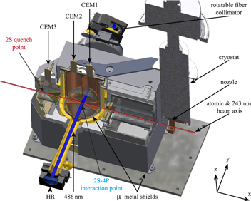
**Figure 2.** Cryogenic 2S beam apparatus and large solid angle detector setup. Atomic hydrogen thermalizes at the inner walls of a copper nozzle which is temperature stabilized to 5.8 K. An atomic beam is collimated from the atoms leaving the nozzle to the left by two diaphragms and excitation of the 1S–2S transition takes place collinear to the atomic beam axis. Excitation of the 2S–4P transition takes place in another separated region. The laser to atomic beam angle is close to 90 ${}^{\circ }$ . Lyman-γ photons which are emitted upon the 4P–1S decay are detected by channel electron multipliers (CEM1 and CEM2) via photoemission of electrons from the graphite coating within the detector region. The 486 nm excitation light polarization is controlled by an optical polarization maintaining fiber fixed on a rotatable collimation system. Compared to [16], an additional detector has been installed (CEM3). In this third region all 2S atoms are de-excited by a static electric field [9]. The detector can be used to measure the number of remaining 2S atoms after the 2S–4P interaction and to normalize the flux of 2S atoms for the reduction of non-Poissonian noise on the other detectors.
Download figure:
Standard image High-resolution image

**Figure 2.** Cryogenic 2S beam apparatus and large solid angle detector setup. Atomic hydrogen thermalizes at the inner walls of a copper nozzle which is temperature stabilized to 5.8 K. An atomic beam is collimated from the atoms leaving the nozzle to the left by two diaphragms and excitation of the 1S–2S transition takes place collinear to the atomic beam axis. Excitation of the 2S–4P transition takes place in another separated region. The laser to atomic beam angle is close to 90 ${}^{\circ }$ . Lyman-γ photons which are emitted upon the 4P–1S decay are detected by channel electron multipliers (CEM1 and CEM2) via photoemission of electrons from the graphite coating within the detector region. The 486 nm excitation light polarization is controlled by an optical polarization maintaining fiber fixed on a rotatable collimation system. Compared to [16], an additional detector has been installed (CEM3). In this third region all 2S atoms are de-excited by a static electric field [9]. The detector can be used to measure the number of remaining 2S atoms after the 2S–4P interaction and to normalize the flux of 2S atoms for the reduction of non-Poissonian noise on the other detectors.
Download figure:
Standard image High-resolution image

The optical excitation of the 2S state provides our experiment with a variety of advantages over the previous optical 2S–nL transition frequency measurements shown in figure 1(a), the most important of which are:

In contrast to electron-impact excitation which has exclusively been used in the other experiments, optical excitation preserves the atom's thermal velocity. Typical mean velocities for 2S atoms excited by electron-impact reside around 4 km s⁻¹ [13]. In combination with the cryogenic source of 1S atoms, we obtain mean velocities of our 2S atoms around 300 m s⁻¹, more than one order of magnitude smaller than that.
It provides a well defined and fast way to discontinue the flux of 2S atoms for time-of-flight resolved data acquisition. Using this technique, ten data sets with atom mean velocities ranging from 270 m s⁻¹ down to less than 70 m s⁻¹ can be acquired in one single shot.
The optical excitation of the 2S state by the narrow band continuous wave laser in our apparatus is state-selective. From the different hyperfine and Zeeman sublevels in the 2S manifold, only the 2S(F = 0) state is populated. This significantly simplifies the excitation dynamics and characterization of the subsequent 2S–4P excitation.

4.3. ${10}^{6}$ suppression of the FOD effect

Although the cryogenic source of 2S atoms reduces the thermal mean velocity of 2S atoms in our apparatus to around 300 m s⁻¹, the full Doppler effect on the 2S–4P transition still amounts to 617 MHz for this velocity, i.e. it has to be suppressed by more than six orders of magnitude to achieve the envisioned uncertainty goal in the low kHz regime. Arranging the excitation light and atomic beam axes to be close to 90° in a practical alignment procedure reduces the effect in a straight forward way to about 1 MHz, assuming a 0.1° uncertainty in the angle determination. For the residual effect to be controlled, more sophisticated methods have to be applied.

We adapted and advanced the idea of exciting the one photon transition with two antiparallel laser beams as has already been used in the 2S–4P measurement of Berkeland et al [13]: if the angle between atomic and exciting laser beam is different from 90°, the FOD effect will lead to a shift that is unknown if an exact angle is not defined. Exciting the transition with two laser beams, though, leads to two observed resonance profiles which are shifted by the same amount to opposite directions in the ideal case of two counter-propagating antiparallel plane waves. Hence, if the waves are of equal intensity, the center of weight of this double peak structure indicates the position of the atomic resonance, free of the FOD effect and independent of the angle of the atomic beam with respect to the excitation light propagation direction.

To establish these antiparallel beams, the light of an optical single mode fiber is collimated by an objective with low imaging aberrations, retroreflected by a high reflectivity mirror and coupled back into the fiber [16]. The amount of light coupled back into the fiber is monitored and is used to actively stabilize the mirror tip and tilt for optimum coupling. The optical single mode fiber not only serves as a small pin hole for the alignment of the retroreflected beam, it also provides spatial filtering of the light interacting with the atomic sample. The distance between the collimation system and the fiber tip is adjusted such that the waist of the resulting Gaussian beam is placed on the plane surface of the reflecting mirror, thus making the wave fronts of forward and backward traveling light exactly match each other.

A possible residual Doppler effect can be characterized utilizing our time of flight resolved detection scheme: after discontinuing the flux of 2S atoms by switching off the 1S–2S excitation light, the mean velocity of 2S atoms contributing to the 2S–4P signal can be adjusted by introducing a certain delay time τ before acquiring the signal, letting the fastest atoms escape the interacting region. In practice, ten independent data sets with mean velocities ranging from 270 m s⁻¹ down to less than 70 m s⁻¹ are being recorded in a single shot by subdividing the signal into ten time intervals. If a residual FOD effect was present in the data due to imperfections of the suppression system, it has to show up as a linear dependence of the extracted atomic resonance frequency versus mean velocity of the contributing velocity class. As illustrated in figure 3 this dependence is largely suppressed by our active fiber-based retroreflector. The residual slope is compatible with zero and limited by statistics, even when averaged for an entire measurement day, as has exemplary be done in the figure.

**Figure 3.** Suppression of the first order Doppler effect (FOD). (a) The experimental uncertainty in the alignment of the angle α between atomic and excitation light beam amounts to $0.1^\circ$ . Red lines indicate the full (uncompensated) first order Doppler effect at $\pm 0.1^\circ$ deviation from the ideal situation where $\alpha =90^\circ$ . Shown in blue are mean values of one measurement day for the extracted 2S–4P ${}_{1/2}$ transitions frequency for different velocity classes (150 line profiles averaged) and in green the extrapolation to zero velocity where any residual Doppler effect vanishes. Experimental errorbars are not visible on this scale. (b) Close-up of the experimental data shown in (a). The extracted slope of −36(25)Hz/(m s⁻¹) is compatible with zero and limited by the statistical uncertainty of the individual data points, suggesting that the cancellation of the FOD in fact works better than may be characterized by this method. Enhanced sensitivity can be achieved by completely switching off the Doppler cancellation in a differential measurement, see text for details.
Download figure:
Standard image High-resolution image

$0.1^\circ $ — **Figure 3.** Suppression of the first order Doppler effect (FOD). (a) The experimental uncertainty in the alignment of the angle α between atomic and excitation light beam amounts to $0.1^\circ$ . Red lines indicate the full (uncompensated) first order Doppler effect at $\pm 0.1^\circ$ deviation from the ideal situation where $\alpha =90^\circ$ . Shown in blue are mean values of one measurement day for the extracted 2S–4P ${}_{1/2}$ transitions frequency for different velocity classes (150 line profiles averaged) and in green the extrapolation to zero velocity where any residual Doppler effect vanishes. Experimental errorbars are not visible on this scale. (b) Close-up of the experimental data shown in (a). The extracted slope of −36(25)Hz/(m s⁻¹) is compatible with zero and limited by the statistical uncertainty of the individual data points, suggesting that the cancellation of the FOD in fact works better than may be characterized by this method. Enhanced sensitivity can be achieved by completely switching off the Doppler cancellation in a differential measurement, see text for details.
Download figure:
Standard image High-resolution image

In order to obtain a conservative result free of any residual Doppler effect, the extracted values for different velocity classes have been extrapolated to zero velocity up to now. With the most recent upgrade of the experiment, we introduced a more effective way to deal with possible imperfections of the Doppler suppression scheme: a remote controlled shutter in front of the high reflecting mirror has been installed. This way, the Doppler cancellation can be entirely switched off during the experiment. For characterization, the suppression factor can now be measured at different angles by the comparison of the slopes with and without the cancellation. For the actual experiment, the measurement of the full Doppler effect with only one laser beam present can used as a highly sensitive alignment tool. In addition to that, a differential measurement with alternating switching of the cancellation can be performed and the previous extrapolation to zero velocity can be replaced by averaging the data corrected for the Doppler effect. This method is expected to improve the statistical uncertainty by a factor of ten at the cost of 50% data acquisition time. Accordingly, our typical one-day statistical uncertainty of 5 kHz per day would decrease to less than 2.5 kHz per day, enabling more accurate and less time consuming checks for systematic effects.

4.4. Quantum interference in spontaneous emission

There is a variety of possible systematic effects, which can influence the final result of our 2S–4P absolute transition frequency measurement. Some of them, like the FOD effect, we believe to be well under control, others are still under investigation. Amongst those, the line shape modifications due to quantum interference in spontaneous emission, also referred to as cross damping, are the most cumbersome. Although this effect is well known and utilized in other fields of quantum optics (see e.g. the phenomena of quantum beats in radiative decay [17]), these effects have been widely ignored in the treatment of precision spectroscopy data. Their importance for precision spectroscopy experiments has recently been pointed out by Horbatsch and Hessels [18, 19]. Shortly thereafter, spectroscopy experiments on the ${}^{\mathrm{6,7}}$ Li D₂ lines demonstrated that the corresponding shifts of observed line center frequencies can render experimental results meaningless if not taken into account properly [20, 21]. The D₂ lines in ${}^{\mathrm{6,7}}$ Li are partially unresolved and the effects of cross damping are particularly strong. In case of our measurement of 2S–4P transition in atomic hydrogen the separation of the relevant neighboring resonances is as large as 100 natural line widths. However, small deviations from the Lorentzian line shape can still shift the extracted line center by an amount critical for the validity of the final result.

For most practical cases, the natural line shape of an atomic resonance is well approximated by a Lorentzian function. This approximation fails in the presence of another nearby resonance or if the line center is to be determined with high accuracy as the following simple—although by far not complete—example illustrates: consider a classical electrical dipole moment performing damped oscillations at two distinct frequencies ${\omega }_{1}$ and ${\omega }_{2}$ . The individual dipole amplitudes ${\vec{d}}_{1}$ and ${\vec{d}}_{2}$ may point in different directions and are assumed to be real by extracting a possible phase φ between them. The observed intensity spectrum is given by the square modulus of the sum of two complex Lorentzian functions, obtained by Fourier transform of the exponentially damped oscillations:

$\begin{eqnarray}&&{\left|\vec{\tilde{d}}(\omega )\right|}^{2}={\left|\displaystyle \frac{{\vec{d}}_{1}}{{\rm{i}}(\omega -{\omega }_{1})+{\Gamma }_{1/2}}+\displaystyle \frac{{\vec{d}}_{2}{{\rm{e}}}^{{\rm{i}}\varphi }}{{\rm{i}}(\omega -{\omega }_{2})+{\Gamma }_{2}/2}\right|}^{2}.\end{eqnarray} \tag{ 3 }$

The resulting sum consists of three contributions, two real valued Lorentzian functions resembling the intensity spectrum of an isolated oscillator at ${\omega }_{1}$ and ${\omega }_{2}$ respectively and a third cross term, which depends on the relative orientation of ${\vec{d}}_{1}$ and ${\vec{d}}_{2}$ and the phase φ between them. The cross term vanishes when ${\vec{d}}_{1}\cdot {\vec{d}}_{2}=0$ , i.e. for orthogonal dipoles.

Historically, when dealing with neighboring resonances in precision experiments, e.g. in the treatment of off-resonant excitation of transitions other than the spectroscopy transition, the resulting line shapes have widely been modeled using sums of real valued Lorentzians, ignoring the effects of cross damping. Figure 4 illustrates the line shifts obtained by fitting a real valued Lorentzian to one of the spectral features in our simple model as a function of the distance of the two resonances in frequency space for ${\Gamma }_{1}={\Gamma }_{2}$ : the black dashed line corresponds to the line shifts expected from a pure sum of two Lorentzians, while the colored lines illustrate line shifts obtained from the Lorentzian fit for the case that the doublet was properly modeled using equation (3). The latter shifts may be orders of magnitude larger than expected from the simple sum of two real valued Lorentzians, especially for large separation of the two resonances. Precise study of the effects of cross damping is mandatory if the line center position is to be found with high accuracy. A helpful rule of thumb is given in [18]: for a determination of the line center with an uncertainty of $1/N$ of the line width Γ, resonances $N\times \Gamma$ away may cause significant influence on the respective line shape.

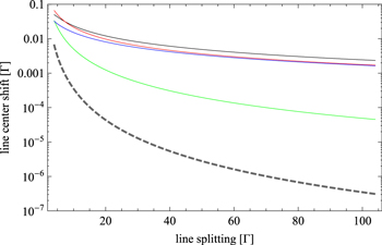
**Figure 4.** Illustration of the line center shifts due to a neighboring resonance. Shown is the line center frequency of one spectral component of a symmetric line doublet ( ${\Gamma }_{1}={\Gamma }_{2}\equiv \Gamma$ , $| {\vec{d}}_{1}| =| {\vec{d}}_{2}|$ ) as a function of line splitting ${\omega }_{1}-{\omega }_{2}$ measured in line widths Γ. Black dashed line: the doublet is modeled by the sum of two real valued Lorentzian functions. Colored lines: the doublet is properly modeled by equation (3), different colors correspond to different phases φ between the dipoles. Especially at large line splitting, the often neglected cross term in the square modulus of equation (3) may lead to shifts which are orders of magnitude larger than the ones expected from the simpler real valued Lorentzian model.
Download figure:
Standard image High-resolution image

${\Gamma }_{1}={\Gamma }_{2}\equiv \Gamma $ — **Figure 4.** Illustration of the line center shifts due to a neighboring resonance. Shown is the line center frequency of one spectral component of a symmetric line doublet ( ${\Gamma }_{1}={\Gamma }_{2}\equiv \Gamma$ , $| {\vec{d}}_{1}| =| {\vec{d}}_{2}|$ ) as a function of line splitting ${\omega }_{1}-{\omega }_{2}$ measured in line widths Γ. Black dashed line: the doublet is modeled by the sum of two real valued Lorentzian functions. Colored lines: the doublet is properly modeled by equation (3), different colors correspond to different phases φ between the dipoles. Especially at large line splitting, the often neglected cross term in the square modulus of equation (3) may lead to shifts which are orders of magnitude larger than the ones expected from the simpler real valued Lorentzian model.
Download figure:
Standard image High-resolution image

For real atomic systems, the description of quantum interference in spontaneous emission is much more complex than for the toy model described in the previous paragraphs. When more than one atomic transition is coherently excited, the decay rates of individual states in the coherent superposition may be modified due to the interaction with the electromagnetic vacuum modes. Detailed description of the underlying theory with special focus on precision spectroscopy experiments can be found in [19, 21–23]. It can be shown that for fluorescence detection, these interference effects lead to shifts in the line center extracted from a simple Lorentzian fit, depending on the geometry of a specific experiment. If the detection solid angle ${\Omega }_{\mathrm{det}}$ of the apparatus is equal to 4π, i.e. all emitted photons are detected with equal probability, the line shape modifications due to interference vanish and modeling the natural line shape by Lorentzians is sufficient. The same is true for detection in a half sphere, i.e. ${\Omega }_{\mathrm{det}}=2\pi$ . On the other hand the effect becomes more pronounced the smaller the detection solid angle is.

For our measurement of the 2S–4P transition in atomic hydrogen, we model the effects of quantum interference in spontaneous emission using two different approaches: the perturbative approach used in [21] and numerical integration of the optical Bloch equations (OBEs) with proper decay constants as described in [19, 22]. While the perturbative treatment can be done analytically and is therefore easy to implement, solving the OBEs for our system requires the numerical integration of more than 2700 coupled partial differential equations for the states involved in the excitation dynamics. The computationally intensive calculations have been performed using facilities provided by the MPG/IPP Rechenzentrum Garching. In addition to the effects of cross damping, the solution of the OBEs can be used to investigate other systematic effects, such as the ac Stark effect, saturation, optical pumping and off-resonant excitation of other levels.

For experimental study of the effects of quantum interference in spontaneous emission, we developed an upgraded version of our large solid angle fluorescence detector, depicted in figure 2. The basic principle of this detector has been discussed before [16]. Excitation of the 2S–4P transition takes place at the crossing point of the atomic and 486 nm laser beam, labeled '2S–4P interaction point', at an angle close to 90°. Lyman-γ photons emitted upon the rapid decay of the 4P state are indirectly detected by channel electron multipliers labeled CEM1 and CEM2. A large detection solid angle is achieved by collecting photoelectrons which are released from the graphite coating on the detector's inner walls by a positive voltage applied to the CEM's input surface. Splitting the detector along the y–z-plane (see figure 2) and rotating the linear 2S–4P excitation light polarization gives rise to a broken symmetry in the signals seen by the two CEMs. The expected shifts of the observed line center positions for each detector as well as the difference are depicted in figure 5 as a function of laser polarization direction. At small excitation light powers of a few μW, the perturbative approach and OBEs give good agreement within the respective uncertainties and the observed shifts are predicted to be in the range of multiple tens of kHz, despite of the large detection solid angle of the detector. Figure 5 also illustrates another feature of the geometry dependence of the interference effect: rotating the linear excitation light polarization in the x–z-plane leads to significant changes in the extracted line center frequency which can be shown to vanish at the 'magic angle' of 54,7° with respect to the symmetry axis of a rotationally symmetric detector [21]. A first signature of this polarization dependent behavior has been observed in the experiment and a more detailed study is underway.

**Figure 5.** Simulated line center shifts due to quantum interference in spontaneous emission for the detector geometry shown in figure 2. The detector is split along the y–z-plane, breaking the rotational symmetry along the z-axis. The two channel electron multipliers CEM1 and CEM2 observe the same instantaneous signal, but at different effective angles with respect to the linear laser polarization, enabling high common noise suppression for the observed difference in signals (green line). We perform simulations for this scheme, using the perturbative approach for the description of the interference effects in spontaneous emission similar to [21] (solid blue lines) and the numerical solution of the optical Bloch equations for the involved states (dashed blue lines). Both of them predict line center shifts of up to several tens of kHz in dependence of the linear excitation light polarization in good agreement within their uncertainties.
Download figure:
Standard image High-resolution image

In addition to the split fluorescence detector, another detector has been installed in the apparatus ('2S quench point' in figure 2). It monitors the number of 2S atoms after the 2S–4P interaction. Observing the decrease in 2S population rather than fluorescence, this detector's signal to noise ratio is inherently worse than the first one. Still, it can give valuable input for the characterization of the cross damping effects, because this way of detection is free of the polarization dependent line shape modifications due to interference. In addition, the detector can be used for normalization of the 2S atom flux, one of the largest non-Poissonian noise contributions in our system, and thereby helps to reduce the noise on the other detector's signals.

4.5. The 2S–6P transition

In addition to the laser systems used for spectroscopy of the 1S–2S and 2S–4P transitions, a third laser system at 410 nm for spectroscopy of the 2S–6P transition is now fully operational in our lab. Its basic design follows the one of the other two systems and has been described in detail in [24, 25]: a long external cavity diode master laser with intra-cavity electro-optic modulator is operating at 820 nm and stabilized to a high-finesse reference cavity made from ultra-low expansion glass. The 40 mW IR output of the master oscillator is amplified in a tapered amplifier and subsequently frequency doubled to obtain the spectroscopy light at 410 nm. The laser frequency is scanned by a double pass acousto-optic modulator in random order and fluorescence photons at 94 nm emitted upon the decay of the 6P state are detected. The resulting resonance profiles are shown in figure 6 for different time windows τ as discussed above. At the incident excitation light power of 200 μW in this case, the observed line width is about 12 MHz, three times larger than the natural line width. Dominating broadening processes are the atomic beam divergence and power broadening.

**Figure 6.** The 2S–6P transition. A first signal from the 2S–6P transition has been obtained at our cryogenic source of hydrogen 2S atoms in February 2014. Depicted are four out of ten line profiles which are recorded simultaneously for different delay times ${\tau }_{j}$ between switching off the supply of 2S atoms and their arrival at the 2S–6P interaction point. The data has been recorded in the same setup that is currently being used for 2S–4P spectroscopy.
Download figure:
Standard image High-resolution image

**Figure 6.** The 2S–6P transition. A first signal from the 2S–6P transition has been obtained at our cryogenic source of hydrogen 2S atoms in February 2014. Depicted are four out of ten line profiles which are recorded simultaneously for different delay times ${\tau }_{j}$ between switching off the supply of 2S atoms and their arrival at the 2S–6P interaction point. The data has been recorded in the same setup that is currently being used for 2S–4P spectroscopy.
Download figure:
Standard image High-resolution image

In a first step, the 2S–6P transition will be used to characterize dc electric stray fields in our apparatus for the absolute frequency measurement of the 2S–4P transition. The corresponding dc Stark effect on the transition of interest scales with the seventh power of the principal quantum number n approximately, giving rise to a 17 fold higher sensitivity of the 6P state as compared to the 4P state. To our knowledge, this will be the first high resolution spectroscopy of the 2S–6P transition in atomic hydrogen. After that, we also plan to measure the absolute transition frequency of the 2S–6P transition and obtain another precise value pair [ ${R}_{\infty }$ , r_p] by combining the result with the 1S–2S transition frequency.

According to the rule of thumb given above, the size of the interference effect is proportional to the ratio of involved states' line widths and separations. The perturbing levels in our experiments are different fine structure components. The ratio of the line widths to line separation $\Gamma (n)/\Delta {\nu }_{\mathrm{FS}}(n)$ is therefore constant for different n in first approximation, because both of them scale with the third power of n. Accordingly, the size of the interference effect relative to the transition frequency decreases with increasing principal quantum number n, such that the knowledge about the effect obtained from 2S–4P spectroscopy should be sufficient for proper characterization at higher n.

5. Conclusion and outlook

For the absolute transition frequency measurement of the 2S–4P transition, the FOD effect is by far the largest systematic effect. We believe that the combination of our cryogenic source of hydrogen 2S atoms with the active stabilization and monitoring methods presented in section 4.3 are sufficient to suppress this effect by more than 10⁶, down to the desired few kHz range. Line pulling effects due to unresolved hyperfine transitions, one of main systematic contributions in the previous measurement of the 2S–4P transition frequency, have been greatly reduced by utilizing state-selective optical excitation to the 2S(F = 0) state. The ac Stark and Zeeman shifts are well under control and within a few kHz uncertainty, too. The effects of line shape modifications due to quantum interference in spontaneous emission and corresponding shifts in the extracted line centers are currently under investigation. As soon as the behavior is understood for our particular geometry and excitation dynamics, the results obtained will be used to minimize the effect in the final data for the extraction of the unperturbed 2S–4P transition frequency.

After the 2S–6P transition has been used to obtain an upper bound for electric stray fields in our apparatus for the 2S–4P experiment, a measurement of the 2S–6P absolute transition frequency is planned. In parallel to that, another laser system for the spectroscopy of the 2S–8P, 2S–9P and 2S–10P transitions is under construction. The combination of these measurements with the 1S–2S transition frequency can provide an improved value for the Rydberg constant as well as a new value for the proton rms charge radius from electronic hydrogen spectroscopy. This will facilitate an improved test of bound state QED in atomic hydrogen and deliver additional input data for the proton size puzzle.

Acknowledgments

Computations have partially been performed using facilities provided by the MPG/IPP Rechenzentrum Garching. KK and NK acknowledge support from DFG HA 1457/101-1 and RFBR 14-02-91331, RP from the European Research Council (ERC) Starting Grant #279765 and TWH from the Max Planck Foundation.

Precision spectroscopy of 2S–nP transitions in atomic hydrogen for a new determination of the Rydberg constant and the proton charge radius

Article metrics

Submit

Permissions

Author e-mails

Author affiliations

Dates

Abstract

1. Introduction

2. QED description of the hydrogen atom

3. The proton size puzzle

4. The hydrogen 2S–4P transition

4.1. The choice of the transition

4.2. Cryogenic source of hydrogen 2S atoms

4.3. ${10}^{6}$ suppression of the FOD effect

4.4. Quantum interference in spontaneous emission

4.5. The 2S–6P transition

5. Conclusion and outlook

Acknowledgments

Precision spectroscopy of 2S–nP transitions in atomic hydrogen for a new determination of the Rydberg constant and the proton charge radius

Article metrics

Submit

Permissions

Share this article

Author e-mails

Author affiliations

Dates

Abstract

1. Introduction

2. QED description of the hydrogen atom

3. The proton size puzzle

4. The hydrogen 2S–4P transition

4.1. The choice of the transition

4.2. Cryogenic source of hydrogen 2S atoms

4.3. {10}^{6} suppression of the FOD effect

4.4. Quantum interference in spontaneous emission

4.5. The 2S–6P transition

5. Conclusion and outlook

Acknowledgments

4.3. ${10}^{6}$ suppression of the FOD effect