Abstract
A watt balance is a precision apparatus for the measurement of the Planck constant that has been proposed as a primary method for realizing the unit of mass in a revised International System of Units. In contrast to an ampere balance, which was historically used to realize the unit of current in terms of the kilogram, the watt balance relates electrical and mechanical units through a virtual power measurement and has far greater precision. However, because the virtual power measurement requires the execution of a prescribed motion of a coil in a fixed magnetic field, systematic errors introduced by horizontal and rotational deviations of the coil from its prescribed path will compromise the accuracy. We model these potential errors using an analysis that accounts for the fringing field in the magnet, creating a framework for assessing the impact of this class of errors on the uncertainty of watt balance results.
Export citation and abstract BibTeX RIS

Original content from this work may be used under the terms of the Creative Commons Attribution 3.0 licence. Any further distribution of this work must maintain attribution to the author(s) and the title of the work, journal citation and DOI.
1. Introduction
The International System of Units (SI) is facing one of the most significant revisions in history. Four of the seven SI base units, the kilogram, the mole, the ampere, and the kelvin, will be redefined by fixing a set of fundamental physical constants, the Planck constant, the Avogadro constant, the elementary charge, and the Boltzmann constant [1]. Before this redefinition can happen in 2018, these physical constants must be determined with sufficient accuracy. Perhaps the greatest challenge in this regard has been the precision measurement of the Planck constant h, since it must be known to within a few parts in 108 in order to afford a seamless transition when redefining the unit of mass, the kilogram [2].
Recently, watt balances [3] that compare electrical power to mechanical power to determine the Planck constant h have demonstrated sufficient accuracy [4], and plans are now in place to begin testing these instruments and their ability to realize a unit of mass [5]. The realization of the unit of mass using a watt balance is conceptually fairly simple, exploiting two functional modes of a specially designed electromagnetic mass balance. First, a weighing mode is completed that measures a test mass by balancing its gravitational force with an opposing electromagnetic force generated from a current-carrying coil in a magnetic field. This force is expressed as mg = BlI where m denotes the unknown mass of the test mass, g is the local gravitational acceleration, which can be measured very precisely using a separate apparatus, B and l are the magnetic flux density at the coil position and the coil wire length, respectively, and their product is an as yet undetermined constant, and I is the direct current through the coil, which is measured in terms of quantum standards of resistance and voltage that allow the weighing current to be expressed in terms of the Planck constant. Next, a velocity mode is completed that measures the product of B and l, known as the geometric factor or flux integral of the coil, so that the value of the mass can be computed from the measured current. The mass is removed in velocity mode and the coil is translated in the magnetic field along a prescribed path with a measured velocity v, inducing an open circuit voltage of U measured across the coil terminals, from which Bl is computed by the voltage-velocity ratio as Bl = U/v.
In contrast to the historical one-phase approach used to establish the relationship between electrical and mechanical units [6], the two-mode measurement of a watt balance eliminates the need to measure current distributions and the detailed physical geometry of the coil magnet system in order to compute the flux integral. As a result, the accuracy of representing a mass at the kilogram level has been improved by 2–3 orders of magnitude, making it accurate enough to become the primary realization in a revised system of units. A more detailed account of the principles and recent progress of watt balance experiments at various National Metrology Institutes (NMIs) can be found in several recent review papers [7–9]. For the purpose of this paper, it is sufficient to appreciate that the accurate determination of the voltage-velocity ratio is key to using the instrument to realize mass, and that an understanding of potential error sources in its determination will be critical to assuring consistency among the growing variety of watt balances that will be used to realize standards of mass around the globe.
The weighing cell of a watt balance, typically either a beam/wheel balance [10–12] or a mass comparator [13–15] must be highly sensitive to forces acting in the direction of gravity. The coil and weighing cell must also accommodate the translation of the coil along this axis, either using the range of motion of the weighing cell, or by translating the entire cell and coil using a specially made stage. In either physical arrangement, the resulting systems are all susceptible to undesired disturbances, such as ground vibrations, that can excite horizontal and rotational motions of the coil that create spurious induced voltages [16] during velocity mode. These voltages are indistinguishable from the voltage induced by the vertical motion, and must therefore be minimized or accounted for through alternate means.
The magnetic field at the coil position can be made one dimensional using properly designed pole pieces (e.g. the 'BIPM' design) to produce a field that decays as 1/r in the horizontal r direction. Parasitic horizontal motions of a circular coil in such a uniform radial field cannot, in principle, induce a voltage. Unfortunately, it is difficult to create a perfectly uniform radial field, and it is far more likely that the field will be two dimensional, particularly near the boundaries of the air gap where fringing will occur [17]. Given these practical considerations, and the need to determine the flux integral with relative uncertainty better than  , we seek an analytical expression for the induced voltage that can aid us in bounding the magnitude of errors given realistic coil motions in a two dimensional magnetic field B(r, z). This type of study is typically referred to as an assessment of misalignment error [18–21].
Assume that the experiment has been well-aligned in the weighing mode, so that
where  is the magnetic flux linkage at the coil position and
  . In order to account for coil motions during velocity mode, the induced voltage can be written as
where vz is the velocity of the coil along the vertical axis z, vx and vy are the horizontal velocities of the coil along the x and y axes;  ,
,  and
and  are the tilt angles of the coil around the x, y, and z axes; and
  ,
,  and
and  are the derivatives of these tilt angles with respect to time. The relative change of the geometrical factor due to misalignments and parasitic motions is condensed to a single constant, ε.
In the remainder of the article, an electromagnetic model is developed to evaluate ε considering static deviations in alignment between coil and magnet, dynamic coil motions, and non-uniformity of the magnetic field. Section 2 begins with the derivation of the magnetic field structure and a general expression of the effect of coil motions on induction. Next, the general model of induction is reduced to consider specific cases. The problem of a coil statically displaced from the symmetry axis is presented in section 3 and then for the dynamic case in section 4. Similarly, static and dynamic coil rotation effects are analyzed in sections 5 and 6. Results of the analysis are summarized and a conclusion are drawn in section 7.
2. General considerations
2.1. Watt balance magnets
There are many types of magnet designs for watt balances, and they may be broadly categorized based on whether the fixed field is provided using field coils [11], permanent magnets [10, 12–14, 22, 23], or more complex electromagnetic systems [24]. The desire to minimize heating of the coil during the weighing mode, and the inevitable change in l which will accompany it, has led designers to balance the trade-offs between number of turns, versus amount of current, versus strength of static field, such that magnetic fields between 0.4 T–1.0 T are typical. Permanent magnets are well suited for this task, and a construction employing two permanent magnets and one coil (shown in figure 1) has become common in the watt balance community, having originated with the watt balance group at Bureau International des Poids et Mesures (BIPM) [25]. The utility of this magnet topology is 1) it yields a nearly 1/r field dependence in the horizontal plane and 2) it provides a horizontal magnetic field that is nearly uniform over the height of the gap. Although our subsequent analysis will employ a magnet and pole geometry of this sort, as shown in figure 1, the model and analysis are general and can be applied to other permanent magnet systems.

Figure 1. A typical magnet structure employed in watt balances. The dashed lines denote the magnetic flux lines.
Download figure:
Standard image High-resolution imageThe watt balance magnet in figure 1 has a symmetrical structure in both the vertical and azimuthal directions. Poles of like polarity on two permanent magnets are set to face each other in symmetrical upper and lower positions of the inner yoke. Their magnetic flux is guided by the inner yoke through a small vertical air gap, and then passes through the outer yoke back to their respective opposite poles. Since the yoke is constructed using materials of high permeability, the majority of the magnetomotive force will drop in the air gap. As a result, a strong, uniform horizontal magnetic field with nearly zero flux in the vertical direction will be generated everywhere in the air gap except for fringing fields at the upper and lower ends [17].
Ideally, all the magnetic flux lines through the air gap are purely radial, independent of z, which is true when the air gap height is infinite. In this case, because the total flux  is a fixed number, the horizontal magnetic flux density through a single vertical surface Br(r) is

Equation (3) shows where r is the radius of the vertical surface and d its height. Equation (B.3) shows that the horizontal magnetic flux density Br(r) falls off with 1/r decay along the r direction. Because the height of the air gap is finite, the magnetic field at a vertical position z in the air gap is only completely horizontal at an imaginary mid-plane, where we set z = 0. Elsewhere, the influence of the upper and lower fringe fields, combined with geometric imperfections in the pole pieces (e.g. non-uniform gap) will lead to asymmetry.
In order to describe the magnetic field in the air gap during velocity mode (I = 0) and better account for asymmetries, the differential forms of the magnetostatic equations in the air gap can be used, where we take advantage of the fact that both the divergence and curl of a magnetic field are zero in the absence of currents and changing electric fields, so

From equations (4) and (5), it is clear that equation (3) holds only at the symmetry plane z = 0 where  and
and  . Outside the symmetry plane, the field has in general a z component. We consider here a magnet that has cylindrical yokes and not specially engineered yokes to extend the 1/r field region.
A three-dimensional map of the magnetic flux density in the air gap is shown in figure 2. The figure indicates that the absolute value of the vertical magnetic field component of the air gap, Bz, increases quickly for values of z departing from the symmetry plane. As a result, the horizontal magnetic component Br will deviate from a 1/r dependence whenever the coil is vertically offset from center.
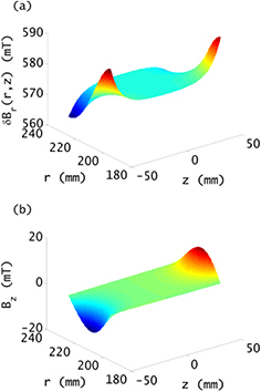
Figure 2. An example of 3D magnetic flux density map in the air gap region of the watt balance magnet. The inner and outer radii of the air gap are 195 mm and 225 mm respectively. The height of the air gap is 150 mm, of which we are interested in the central 100 mm. (a) The  profile where
  mm is the middle radius of the air gap. (b) The Bz(r, z) field contribution in the air gap. A detailed simulation parameter setup can be found in [17].
Download figure:
Standard image High-resolution image2.2. General expressions of the coil motion effect
All discussions in this article are based on the assumption that in weighing operation of watt balances, the coil is not tilted and its center is located in the center of the magnet (x = 0, y = 0, z = 0). The mean radius of the coil  is in the center of the air gap.
In the weighing mode, the coil position should be adjusted to be insensitive to the current through the coil. To keep the equations simple, the coil is assumed to be a single turn coil and its geometrical factor in weighing mode (Bl)w = mg/I is given as

where  denotes the horizontal component of the magnetic flux density at the weighing position. In the velocity mode, considering the coil dynamics, a full expression of a potential voltage U across a conductor (the coil) when it is moving in the magnetic field
  can be expressed as
The velocity vector  and the magnetic flux density vector
  in (7) are written in three dimensional forms as
  and
and  , where vx, vy, vz and Bx, By, Bz are the components in x, y and z directions. In the analysis, the origin of the coordinate system is at the coil center and the coil is assumed to be perfectly circular, thus the vector
  can be expressed as
  . Hence the integral in equation (7) can be expressed as
Thus the geometrical factor  in the velocity mode is calculated as
Comparing equations (6) and (9), the systematic effect ε defined in equation (2), can be written as
There are three terms in equation (10). The first two terms,

describe the dependence of the flux integral from the coil position and orientation. In principle the coil position can be different in the  and the
  direction, where
  denotes a rotation of the coil around the axis i. During the velocity mode the coil sweeps along z and a measurement of Bl(z) is made. From this measured profile of Bl as a function of z the value at the weighing position z = 0 is obtained by fitting a high order polynomial function to the measured values. Hence, we can disregard a dependence of Bl from z, because this dependence is taken care of in this fitting procedure. In addition, we assume the coil to exhibits perfectly azimuthal symmetry and hence there is no dependence on
  . The term
  collects the relative change in Bl caused by static displacements along the remaining two translational and two rotational degrees of freedoms. We call this the static error and divide it again in two terms, the coil horizontal displacement (
 ) and the coil tilt (
 ).
).
The third term on the right-hand side of equation (10) is due to the coupling between the coil horizontal velocity and the magnetic vertical component. Because the coil motion gives rise to this term, we call it the dynamic error, given by
Again, this term can be split into a purely translational part ( ) and a purely rotational part (
 ).
).
2.3. Combining the error terms and the relative systematic effect for h
Typically, during a velocity sweep, unwanted coil displacements and motions occur simultaneously. In this article two types of displacement, a horizontal shift and a tilt, and two types of motions, a horizontal velocity and an angular velocity are analyzed. These four contributions to a bias in the Bl measurement in the velocity mode are analyzed independently. However, because the effects are small, the combined effect can be obtained by a simple sum:
The measurements in the velocity mode yield  , where (Bl)v0(z) is the flux integral in the velocity mode in absence of parasitic motions. In the end, the value at the weighing position, typically z = 0 must be obtained by fitting the profile [18]. Performing a Taylor expansion of the parasitic term about z = 0 yields
The higher order terms will influence the shape of the obtained profile, but the value for Bl obtained at z = 0 only depends on  , i.e.

The watt balance is used to measure the Planck constant h. To calculated the effect of ε on h, we take the ratio of (Bl)v0 to (Bl)w and write each quantity of Bl as the product of its numerical value and its natural unit. The numerical value is denoted by  . The natural unit x for Bl obtained in weighing mode is
  , where
  denotes the conventional ampere and in velocity mode is
  , where
  denotes the conventional voltage.
In the absence of parasitic motions the ratio of (Bl)w to (Bl)v0 is unity, because both modes measure the same physical quantity, the flux integral, hence
The ratio of the conventional watt,  , to the SI watt,
  , is the ratio of the Planck constant h to the Planck constant
  Js derived from the conventional electrical units. Hence,
here h denotes the SI value of the Planck constant, which is unknown to the experimenter. The experimenter measures (Bl)v and calculates the ratio given by
The measured value hm of the Planck constant is given by,
In summary, the presence of parasitic coil displacements and motions causes a relative difference between the measured Planck constant and the true Planck constant given by  .
.
3. Static horizontal displacement
In this section, we discuss the effect of the coil not being concentric with the yokes of the magnet. As shown in figure 3, the coil center O (0, 0, z) is set as the reference point, and the position of the magnet center M  where
where  and
and  are the coil displacements in x and y directions and
  is the horizontal displacement of the coil. P
  is an arbitrary point on the coil at an angle θ in the coil coordinate system, given by x and y. The magnetic flux density components Bx and By at point P can be expressed as
where  is the angle between Br and Bx.

Figure 3. A top view of the horizontal coil motion in the air gap. M is the magnetic center, i.e. the center of symmetry of the magnet, while O is the coil center. The coordinate origin is set at the coil center O (0, 0, z) and the magnet center M is ( ).
).
Download figure:
Standard image High-resolution imageFirst, we analyze the effect with the coil vertically in the center of the magnet (z = 0). Here, the horizontal magnetic field component Br follows a 1/r decay along the horizontal direction r, i.e.  , therefore, the components of the magnetic flux densities Bx and By at point P are calculated as
Then the static effect,  , due to the coil displacement can be calculated based on equation (11) as
It can be shown that the integral on the right-hand side of equation (23) equals to 1 (see appendix  . In summary, a coil in a radial field will always produce the same flux integral, independent of its horizontal displacement. A similar conclusion has been also obtained in [21].
Next, we analyze the static effect of a horizontal coil displacement when the coil is no longer in the symmetry plane of the magnet. An actual magnetic profile  in figure 2(a) shows that the shape difference between the actual Br and the ideal 1/r dependence field increases fast for increasing
  .
.
Here, we present an analytical model to express the change in flux integral caused by a horizontal displacement of the coil. A combination of equations (11) and (21) yields
Without loss of generality, the function Br(r, z) can be expressed as a Laurent series in r, or
where  is the coefficient of the Laurent series expansion. The coefficient an is in general a function of z, i.e.
  . For z = 0, B(r, 0) = a−1/r while an = 0 at
  . Substituting equation (25) into equation (24),
  yields
The simplification of equation (26) can be found in appendix
The result is proportional to the square of the dimensionless quantity  . The proportionality constant equals to the sum of coefficients
 ![${{\kappa}_{n}}={{a}_{n}}\left({{n}^{2}}-1\right)r_{\text{c}}^{n}/\left[4{{B}_{r}}\left({{r}_{\text{c}}},0\right)\right]$](https://content.cld.iop.org/journals/0026-1394/53/2/817/revision1/metaa11efieqn062.gif) . Like the coefficient an,
. Like the coefficient an,  is a function of z, while
  and
and  are independent of z. Hence,
  is a one-dimensional function of z.
To evaluate the value of  , all summands
  can be obtained by fitting Br(r, z) with equation (25). However, it can be shown that the series
  does not converge. A direct solution of
  can be found and equation (26) can be written as
Equation (27) shows that the amplitude of the effect from static, horizontal coil displacement at any vertical portion of the coil, i.e.  , can be obtained from the function
  .
.
Results of calculations of f and  based on a finite element analysis of the magnet are shown in figure 4. The top graph shows f as a function of r and z. The lower plot shows
  as a function of z for three different coil diameters. The curve is very flat in a neighborhood of z = 0.
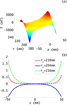
Figure 4. The Bl change due to horizontal movement of the coil when the fringe effect of the magnetic field is considered. (a) 3D mapping of the function f in a full focused air gap region where  (-50 mm, 50 mm),
  (195 mm, 225 mm). (b)
  as a function of z with different coil radii.
Download figure:
Standard image High-resolution imageFigure 4 shows that the coefficient  introduced by the fringe field has a zero value at the vertical center z = 0. This verifies our analysis for
  . The absolute value of
  increases fast when the coil is far from the vertical center. A positive sign of
  means this effect will make the Bl larger when the coil is not centered with the magnet. The calculation shows that
  evaluates to 0.65 at
  mm due to the fringe field.
Figure 4(b) also shows the other two coil dimensions when the coil is designed off center of the air gap,  mm and
  mm. It can be seen that the Bl change can be both negative and positive, depending on the coil radius. Choosing
  to be the same as the radius of the air gap center will reduce the quadratic effect from coil displacements.
4. Dynamic horizontal displacement
In the plane of vertical symmetry z = 0, the vertical magnetic flux density component is 0 and hence  . In the remainder of this section, we discuss the dynamic error
  when the coil is offset from the vertical center, i.e.
  .
.
Similar to the coil displacement analysis, the vertical magnetic flux density in the air gap Bz(r, z) is expressed in power-series form as
where  is the coefficient of the power-series expansion. Based on equations (12) and (28),
  is solved as
The simplification of equation (29) is attached in appendix
Similarly to equation (27), the coefficient of  can also be calculated by a functional approach, i.e.
Based on equation (5),  can be replaced by
  leading to
Equation (31) shows that the functional shape of  is partially determined by the derivative
  in the air gap horizontal center
  . Since the
  is measured in the velocity mode of a watt balance, and hence the value of
  can be easily calculated or directly measured by a gradient coil [22]. A calculation of the coefficient
 ![${{c}_{2H}}=-{{\left(\partial {{B}_{r}}/\partial z\right)}_{r={{r}_{\text{c}}}}}/\left[2{{B}_{r}}\left({{r}_{\text{c}}},0\right)\right]$](https://content.cld.iop.org/journals/0026-1394/53/2/817/revision1/metaa11efieqn100.gif) is shown in figure 5. It can be seen that the absolute value of c2H is about
is shown in figure 5. It can be seen that the absolute value of c2H is about  mm−1 at
  mm while much smaller around the central vertical measurement interval. The absolute value of c2H would increase if the coil radius is designed to differ from the radius of the center of the air gap.
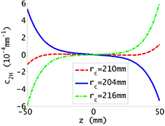
Figure 5. Calculation result of the coefficient ![${{c}_{2H}}=-{{\left(\partial {{B}_{r}}/\partial z\right)}_{r={{r}_{\text{c}}}}}/\left[2{{B}_{r}}\left({{r}_{\text{c}}},0\right)\right]$](https://content.cld.iop.org/journals/0026-1394/53/2/817/revision1/metaa11efieqn103.gif) as a function of z with three different coil radii.
as a function of z with three different coil radii.
Download figure:
Standard image High-resolution imageThe calculation of c2H and equation (31) clearly shows the effect caused by a coil horizontal velocity in consideration of the vertical magnetic component Bz(r, z). Typically, the ratio of the horizontal velocity to the vertical velocity is much smaller than  and the horizontal displacement is less than several μm. Then, the value of
  is of order 10−5 mm, and hence
  , about 20 times smaller than the total relative uncertainties of the best watt balances.
5. Static coil tilt
Other effects stem from the rotation of the coil. We use the word tilt for coil rotations around x and y axes. The tilt can be static, independent of time, or dynamic, leading to angular velocities  and
and  . Here, we discuss the effects of a static tilt.
As shown in figure 6, the coil is titled by an angle of  from the xy plane. S is the point on the coil with a maximum vertical displacement and S' is its projection on the xy plane.
  and
and  are two components of
  which are perpendicular to the x- and y- axes respectively. In figure 6, P is an arbitrary point on the coil and P' is its projection on the xy plane. We assume the angle xOP' is φ, and then the vertical coordinate of P can be written as the sum of two tilt components, i.e.

where lx and ly meet


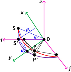
Figure 6. A side view of the rotational motion of the coil in the air gap. O is the center of the coil. S' and P' is the projection of S and P on the xy(ij) plane. Note that in the analysis, a pure coil tilt is assumed, i.e. the coil center is at the magnetic center M.
Download figure:
Standard image High-resolution imageCombining equations (32)–(34) yields
where  . The two rotational components
  and
and  can be optically measured with an autocollimator or an optical lever. Since the point S has a maximum vertical value,
  is calculated as
For easier analysis, we rotate the x and y axes about the z axis by the same angle  . The rotated axes are marked as i and j. In the ij plane, the projection of S, S' is along axis i. P is an arbitrary point on the coil and P' is its projection on the ij plane. We assume OP' = lp and the angle iOP' is θ, and then the coordinate of P can be written as
  . As OP
  , lp can be solved as
where the + sign is chosen because here lp denotes the length of OP'. A change in Bl due to a static coil tilt can arise from two effects. First, the projection effect of the coil, where the projection of the coil on the ij plane is compressed into an ellipse, and hence the equivalent radius of the coil is getting smaller. Second, the vertical magnetic non-linearity, where the coil has a displacement in the vertical direction z, and the difference between Br(z) and Br(0) must be considered. We write the relative change in Bl as a product of two factors that differ from 1 by  and
and  . Hence,

To calculate  , the coil projection to the xy plane is no longer a circle, therefore, we need to modify the basic equation (10). If P' (i, j, z) is an arbitrary point in the projection track, i and j are expressed as
For a static coil rotation, the vector  is written in three dimensions as
To calculate the projection effect, we neglect the z component of  . Integrating
  along
along  according to equation (7), results in
Because pure tilt, without translation, is assumed equation (41) can be simplified using  and
and  to
to
Using the Laurent series expansion of B(r, z) along the vertical direction according to equation (25) we obtain
A detailed simplification of equation (43) is included in appendix  . This independence of Bl on the z = 0 plane verifies our analysis in section 2. Note that equation (43) is a particular case of the result given in [21].
The factor  is due to a non-linear change in Br(z) as a function of z. The vertical coordinate of point P, compared to the coil center z, differs by
The relative change in Bl due to this effect is given by
To evaluate equation (45), the function Br(r, z) is written as a power series in z as
where  is the coefficient of the power series expansion. Substituting equation (46) into equation (45) with a simplification (see appendix
  is obtained as
The vertical non-linearity  can be considered as a one dimensional function of z and independent of the coil horizontal displacement. Because under consideration of the fringe effect, the field gradient of Br(r, z), e.g.
  , can be approximated by the average of horizontal gradient values
  and
and  where
where  is the coil horizontal displacement [17]. Therefore, in calculating
  , the central magnetic profile
  can always be used, without considering the coil horizontal displacement.
According to equations (43) and (47),  and
and  are both functions of
  . In order to evaluate the static error
  , a numerical calculation of the coefficients
  and
and  in the air gap region has been shown in figure 7.
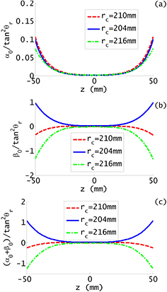
Figure 7. Calculation results of two coefficients: (a)  , (b)
, (b)  and (c)
  .
.
Download figure:
Standard image High-resolution imageFigure 7 shows that the absolute values of  and
and  increase towards both ends of the vertical measurement interval. For
  mm and
  mm, the value of
  is 0.1 and that of
  about −0.25. The latter has a larger value at the vertical ends of the air gap. Since the signs of these two coefficients are opposite at vertical ends, the absolute value of
  is smaller than the absolute values of
  and
and  .
.
Figure 7 also shows values of the coefficients  and
and  when the coil size differs from the mean radius of the air gap. In this case, the value of
  is getting a little smaller while the absolute value of the vertical non-linearity
  is increased, but still not much larger than 1.
The absolute value of  is, under reasonable assumptions, between 0.1 and 1. Hence, a tilt angle of 100 μrad would yield a relative change in Bl that is between 10−9 and 10−8. Overall this is not an obstacle for watt balances, since the coil angle can be measured with an uncertainty of
  1 μrad, hence if there is a small effect it can be corrected such that the overall uncertainty is completely negligible in the reported result.
6. Dynamic coil tilt
In the following, the effect of a changing tilt, i.e. a coil with angular velocity, on the Bl is discussed. For an arbitrary point P on the coil, its two horizontal velocity components are written as

where  and
and  are the angular velocities around the x and y axes. An additional vertical velocity change
  is obtained as

It has been shown in section 5 that the Bl change due to the coil tilt is a quadratic effect of the coil tilt angle  . Therefore, the additional Bl change due to the vertical velocity change can be described as
It can be shown that  , where
  is a sum of higher order terms of
  (
( ). Therefore, the vertical velocity change is averaged out and can be ignored. The relative change in Bl from coil rotation,
  , is mainly given by the product of the horizontal velocity and the vertical magnetic flux density,
Combining equations (28), (48) and (51) yields
Equation (52) is very similar to equation (31), where  ,
,  ,
,  , and
, and  are comparable to
  ,
,  , vx and vy. The dynamic error
  due to the coil rotation is related to two ratios:
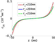
 ![${{c}_{2R}}=-{{B}_{z}}\left({{r}_{\text{c}}},z\right)/\left[2{{B}_{r}}\left({{r}_{\text{c}}},0\right){{r}_{\text{c}}}\right]$](https://content.cld.iop.org/journals/0026-1394/53/2/817/revision1/metaa11efieqn180.gif) ,
,  . The calculation result of the first ratio, c2T, is shown in figure 8. The functional shape of c2T is very similar to that of c2H shown in figure 6, i.e.
  . Figure 8 shows that c2T has a maximum value about
  mm−1, to ensure
  is lower than
  ,
,  should be smaller than
  mm. Note that the c2H value will become a little lower when the coil radius is either smaller or larger than the radius of the air gap center.
Figure 8. Calculation result of the coefficient ![${{c}_{2R}}=-{{B}_{z}}\left({{r}_{\text{c}}},z\right)/\left[2{{B}_{r}}\left({{r}_{\text{c}}},0\right){{r}_{\text{c}}}\right]$](https://content.cld.iop.org/journals/0026-1394/53/2/817/revision1/metaa11efieqn188.gif) as a function of z.
as a function of z.
Download figure:
Standard image High-resolution image
7. Discussion and conclusion
This article summarizes the effect of error motions of the coil on the measured flux integral in a watt balance using a 'BIPM' type magnet system. The Bl obtained in velocity mode differs from the one obtained in the force mode due to a different coil position or parasitic (angular) velocities. The relative change is denoted  Four different scenarios were investigated: a static horizontal displacement of the coil, a horizontal velocity of the coil, a static tilt of the coil, and an angular velocity of the coil. The relative changes in Bl caused by the four types of parasitic motions are denoted,
  and
and  , respectively.
The BIPM type magnets are designed to be up-down symmetric, leading to a horizontal magnetic field Br(r, 0) in the center of the magnet that follows a 1/r dependence. In this case, all four relative changes to Bl vanish,  .
.
At locations away from the symmetry plane  , the 1/r dependence will not strictly hold and the ε will assume small but non-zero values. The detailed derivations of the relative changes in Bl are detailed above. The results can be summarized as follows
The most important aspect of the above equations is that the relative changes in Bl are all second order in the variables describing the error motion. The static horizontal change depends  , where
  is the displacement of the coil from its position in the weighing mode. The dynamic horizontal effect depends on the product of the horizontal velocity and the horizontal displacement, for example,
  . The static tilt depends on the square of the tilt angle
  (for small angles
  ). And finally the dynamic tilt depends on the product of tilt angle and angular velocity, e.g.
  .
.
For the static displacement, the error variable is normalized by the coil radius,  . Hence, a large coil radius is beneficial. On a coil with radius of 200 mm, a displacement of 20 μm leads to
  . Because, the multiplicand in equation (53) is of order 1, the relative error incurred by this relative large displacement is only about 10−8.
As mentioned above, the effects vanish if the radial component of the magnetic flux follows a 1/r dependence. Designing a magnet system, one should try to make the region where  as large as possible. In addition, to reduce the effect of the horizontal velocity of the coil, it is beneficial to make the profile as flat as possible reducing
  . To reduce the effect of a dynamic tilt, the z component of the field should be kept as small as possible. This is also achieved by making the profile as flat as possible.
Symmetry is an important property in the watt balance experiment. In this article we could show that error motions of the coil change the measurement of the flux integral in the velocity mode by a very small amount (of order 10−8) when the magnet system has two basic symmetries: 1) The radial component of the magnetic flux is inverse proportional to the radius at the center plane; 2) The magnet is up-side down symmetric about the center plane.
If the effect of the error motions are not tolerable in the final uncertainty budget, corrections for it can be calculated and applied. Therefore the position of the coil must be monitored during the velocity sweep. This can be done easily using optical readout.
Acknowledgment
S Li acknowledges support from the National Natural Science Foundation of China, grant #51507088.
Appendix A
It can be seen in figure 1 that  and
and  where
where  is the angle between
  and
and  . Then the integral in equation (23) can be simplified as
Since the integral is over a full period, equation (A.1) can be calculated as
Substituting  into equation (A.2), we have
It is equivalent to replace  and the integral interval
 ![$\left(0,\pi \right]$](https://content.cld.iop.org/journals/0026-1394/53/2/817/revision1/metaa11efieqn211.gif) in equation (A.3) with
in equation (A.3) with  and
and ![$\left(0,2\pi \right]$](https://content.cld.iop.org/journals/0026-1394/53/2/817/revision1/metaa11efieqn213.gif) respectively, and hence
respectively, and hence  is rewritten as
A comparison of the beginning row of equations (A.2) and (A.4) yields
In watt balances,  is only a few μm and
  is typical about 200 mm, hence
  is very small. As
  , we have
  , and hence the integral in equation (23) approaches unity.
Appendix B
A general expression of  based on equations (24) and (25) is
Using  and
and  , equation (B.1) is rewritten as
The integral is over one period, and hence  is independent to
  . Then equation (B.2) turns to
As discussed,  is a small number, thus it is reasonable to express the integral term of
  using only the linear and quadratic terms of
  . Obviously, the integral of the linear term, i.e.
  , is zero over one period
 ![$\left(0,2\pi \right]$](https://content.cld.iop.org/journals/0026-1394/53/2/817/revision1/metaa11efieqn229.gif) . Using
. Using  , the integral of the quadratic term is
  and therefore
  is solved as
It has been shown in section 3 that  , i.e.
  when
when  on the vertical center plane z = 0. Obviously, this case (n = −1) also satisfies equation (B.4).
Appendix C
Applying  ,
,  ,
,  ,
,  , where
  is the combined horizontal velocity and
  is the angle between vr and vx, equation (29) can be rewritten as
The integral of the first term  over one period is zero.
  can then be approximated by integrating the linear term of
  , namely
Substituting  ,
,  ,
,  ,
,  in equation (C.2) yields
Appendix D
For the coil projection on xy plane, the radius is lp, thus equation (42) should be calculated as
Substituting equation (37) into equation (D.1) and ignoring higher order terms, the integral term is  , and
, and  is therefore written as
Appendix E
Substituting equation (46) into equation (45) yields
where  is expressed as in equation (44). Then equation (E.1) is rewritten as
The integral of equation (E.2) can be written in polynomials of  as
as
where χ is the higher order terms of  . As the first term of equation (E.3) equals zero,
  is calculated as