

Abstract
This work presents the self-consistent modeling of micro-plasmas generated in dry air using microwaves (2.45 GHz excitation frequency), within capillaries (<1 mm inner radius) at low pressure (300 Pa). The model couples the system of rate balance equations for the most relevant neutral and charged species of the plasma to the homogeneous electron Boltzmann equation. The maintenance electric field is self-consistently calculated adopting a transport theory for low to intermediate pressures, taking into account the presence of O− ions in addition to several positive ions, the dominant species being O , NO+ and O+ . The low-pressure small-radius conditions considered yield very-intense reduced electric fields (∼600–1500 Td), coherent with species losses controlled by transport and wall recombination, and kinetic mechanisms strongly dependent on electron-impact collisions. The charged-particle transport losses are strongly influenced by the presence of the negative ion, despite its low-density (∼10% of the electron density). For electron densities in the range (1–
 cm−3, the system exhibits high dissociation degrees for O2 (∼20–70%, depending on the working conditions, in contrast with the ∼0.1% dissociation obtained for N2), a high concentration of O2(a) (∼1014 cm−3) and NO(X) (
 cm−3) and low ozone production (<
 ).
).
Export citation and abstract BibTeX RIS
1. Introduction
Research in micro-plasma sources has known a growing interest over the last years due to their various potential applications in several fields, such as photonics with the development of powerful UV sources [1], materials with the synthesis of nanostructures [2, 3], micro-propulsion [4], chemical analysis and sensing [5, 6], environmental issues [7], and biomedical applications due to the production of chemically active species [8–11], especially if the plasma is produced in air and under controlled microfluidic flow conditions [12]. Usually, the generation of micro-plasmas (i.e. non-equilibrium plasmas confined to dimensions below 1 mm) is performed under atmospheric-pressure conditions, thus resulting in the production of chemically reactive species through a combination of heavy-species kinetic mechanisms and boundary-dominated phenomena [13, 14]. However, if technically possible, the generation of micro-plasmas at pressure conditions different than atmospheric can be also of practical interest. Indeed, the very-intense excitation predicted by the pd scaling in this case will favor both the emission of energetic radiation and the production of highly-reactive species, two main ingredients for biological applications [8, 15]. Moreover, in a context where standard working conditions are to be modified, the use of surface-wave discharges [16–18] is of particular interest since they ensure a flexibility of operation [19] in terms of wave frequency (from ∼100s of kHz to 10s of GHz), gas pressure (∼10−4–104 Torr), power (∼1–103 W), dimensions (∼10−4–10 m) and geometry (e.g. planar and cylindrical).
This work studies microwave-sustained micro-plasmas in dry air ( ), produced using a surface-wave (SW) excitation (
 GHz frequency) within a small radius capillary (R = 345 μm) at low pressure (p = 300 Pa). The micro-plasmas are characterized using both self-consistent modeling and experimental diagnostics, and the main results of the study are presented in two cluster papers. The present paper is devoted to the self-consistent modeling of the system, discussing the theoretical formulation adopted, its numerical implementation, and the simulation predictions for the different model quantities, as a function of the electron density. The experimental investigation of the micro-plasmas is presented in a companion paper [20], which shows the experimental setup and the optical emission spectroscopy diagnostics adopted, assessing the validity of the model by comparing simulations and measurements under typical working conditions, as a function of the coupled power and the position along the plasma column.
In principle, the modelling of a low-pressure plasma excited by a high-frequency electric field can adopt a stationary description, since it is expected that  [21, 22], with
  the total electron–neutral collision frequency and me / M the electron-to-heavy-species mass ratio. These inequalities reveal that the times for the electron particle / energy relaxation and the electron transport evolution, respectively, are much longer than the oscillation period of the applied electric field, thus showing that the problem is of direct-current (DC) nature even for its most mobile species.
Note that the total electric field experienced by the plasma is  , with
  the space-charge electrostatic field (V being the corresponding potential) and E the high-frequency field. In the case of a plasma column axially-excited within a cylindrical tube, the electrostatic field is aligned mainly in the radial direction, except near the column end where a charge separation in the axial component can also develop. Therefore, the DC radial description of the charged-particle dynamics (balance and transport) involves only the electrostatic space-charge field (or potential), yet connected to the description of the electron energy balance where the DC component of collisional heating involves the high-frequency field [22]. In this work, the balance of energy for the electrons is set by solving the homogeneous two-term electron Boltzmann equation (EBE) for given values of the high-frequency electric field, the excitation frequency, the gas temperature and the ionization degree. The solution to the EBE, for the excitation conditions considered, yields the electron energy distribution function (eedf) that can be used to calculate the electron transport parameters and rate coefficients needed for the description of the charged-particle dynamics.
The unusual small-radius, low-pressure extreme conditions adopted here introduce new modeling challenges, for example as compared to studies developed for discharges with tube radii of the order of the cm. The major consequences are twofold: (i) the development of a very-high maintenance electric field, to compensate for the enhanced radial losses, which can pose some technical problems in the evaluation of the eedf at high kinetic energies; (ii) the need for an adequate description of the charged-particle radial transport, valid for the pR < 0.08 Torr cm conditions adopted here, where the classical ambipolar theory fails.
A careful review of the existing transport theories for charged particles was made by Phelps [23], who clarified the transition from low pressure (collisionless plasma) to high pressure (collisional plasma), and from low electron-density (independent field-free motion) to high electron-density (ambipolar motion). Figure 1 presents a schematic that summarizes these transitions. Here, the transition from low to high pressure is characterized by the ratio  , where
  is the characteristic diffusion length for infinite cylindrical geometry and
  is the ion mean-free-path; whereas the transition from low to high electron-density is associated with the ratio
  , where
  is the Debye length. The high-pressure case (
 ) was treated first by Schottky [24], who deduced the classical ambipolar diffusion coefficient Da, by considering electrons in Boltzmann equilibrium with the electrostatic potential and a single type of positive ions with non-inertial behavior. In this high-pressure range, Allis and Rose [25, 26] derived an effective diffusion coefficient dependent on the ratio
  , to account for the transition between ambipolar and independent motion. The low-pressure ambipolar range (
 and
and  ) was explored first by Tonks and Langmuir [27], who described the so-called free-fall regime by considering electrons with a Boltzmann distribution and a single type of positive ions with inertial motion. A unified transport theory for dense plasmas (
 ) was later proposed by Self and Ewald [28], who combined the transport equations of electrons and ions to describe a plasma column controlled by ambipolar motion at various gas densities, thus bridging the gap between the low and high pressure regimes in a continuous way. The results of Self and Ewald were later expressed by Ferreira and Ricard [29] in the convenient form of another effective diffusion coefficient Dse, introduced so as to extend the Schottky condition to all pressures as
  (with ν the electron net creation frequency). As expected, the value of Dse depends on the ratio
  , giving
  at high pressure and
  as the pressure decreases.
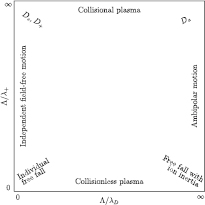
Figure 1. Map of transport regimes, according to the transitional parameters  (representing the gas pressure) and
  (representing the electron density). Based on an idea by A Phelps [23].
Download figure:
Standard image High-resolution imageIn principle, the results presented in [28, 29] for  versus
  could be used at intermediate/low pressures (
 ) to describe the transport of charged particles in the present case. However, the values of Dse proposed by Ferreira and Ricard were obtained for a single type of positive ions and no negative ions, whereas the present study addresses N2-O2 mixtures in the presence of several positive ions and at least one negative ion, which demands a revision of these results in order to fit our working conditions.
The presence of negative ions introduces additional problems when revising the transport theory. Indeed, depending on their density and temperature, negative ions modify the electrostatic space-charge potential, remaining confined to the plasma core due to their low mobility and influencing the radial diffusion length of all other charged particles. In principle, the transport of charged particles can be described by solving numerically the full set of continuity and momentum equations for electrons and ions, as it was done by Edgley and Von Engel [30] for the general case of an arbitrary pressure. However, the approach is hard to implement and the results obtained are not easily translated into a simplified diffusion theory, which explains why other authors have chosen to adopt some extra assumptions, such as the quasi-neutrality condition [31–33] or the imposition of a particular negative ion profile [34]. The work of Ferreira [31] restricts the validity range of Edgley and Von Engel's model to intermediate/high pressures, by assuming quasi-neutrality and by neglecting the positive-ion inertia. A generalization of this formulation to the case of several positive ions is presented in [35]. Conversely, Franklin [32, 33] analyze the low-pressure asymptotic limit by neglecting all collisional processes, thus abandoning the possibility of generalizing the unified transport theory proposed by Self and Ewald. The assumption of a constant density ratio between negative ions and electrons was introduced by Rogoff [34]. The resulting transport description becomes much simpler to handle, but the assumption is valid only if the attachment / detachment rates are large when compared with the ionization rate.
In this work, we revise the unified transport theory proposed by Self and Ewald [28], keeping the assumptions of quasi-neutrality and flux conservation, but considering the presence of several positive ions and the O− negative ion with low density (see table 1). The study is limited to the region of low/intermediate pressures ( Pa), for which the negative ion has negligible drift velocity, remaining confined to the plasma core [32, 33]. Under these hypotheses, it is possible to retrieve a system of equations formally identical to the one of [28], whose numerical solution can be avoided using the results of [29] as an abacus. Even with this correction upon the effective diffusion coefficient Dse, the self-consistent maintenance electric field is expected to continue exhibiting considerably high values. Therefore, the electron cross sections and the corresponding kinetic calculations are extended up to 1000 eV, to describe the effect of the high-energy mechanisms impacting significantly on the tail of the eedf.
Table 1. Summary of the species considered in the model.
| Species | |
|---|---|
| e | |
N2(X, –59) –59) |
O2(X) |
| N2(A) | O2(a) |
| N2(B) | O2(b) |
| N2(C) | O(3P) |
| N2(a) | O(1D) |
| N2(a') | O3 |
| N2(w) | O |
| N(4S) | |
| N(2D) | |
| N(2P) | |
| NO(X) | NO2(X) |
| NO(A) | NO2(A) |
| NO(B) | |
| N+ | O+ |
N (X) (X) |
O |
N (B) (B) |
NO+ |
N |
O− |
 |
|
The organization of this paper is the following. Section 2 describes the theoretical formulation implemented in the numerical code, detailing the transport theory and the kinetic model adopted. The presentation of the latter focuses on a revision upon the electron-scattering cross sections and the kinetic scheme for the ions, for which detailed tables are presented in appendix. Section 3 introduces the numerical code developed, presenting its work-flow and convergence criteria. Section 4 is dedicated to the presentation and discussion of simulation results, focusing on the analysis of the charged-particle transport at various radii and on calculations, as a function of the electron density, of the concentrations and the creation / destruction rates of the main plasma species. Section 5 concludes.
2. Theoretical formulation
The present study focuses on microwave-sustained micro-plasmas in dry air ( ) produced under the following typical working conditions: excitation frequency
  GHz, tube radius R = 345 μm, gas pressure p =300 Pa, gas temperature
  K, electron density
  cm−3, and electron temperature (defined as 2/3 of the electron mean energy)
  –7 eV. For generality sake, in a non-equilibrium situation the electron temperature can be replaced by the electron characteristic energy
  , with De and
  the corresponding electron free-diffusion coefficient and mobility, respectively.
For the purpose of this work, we have developed the LoKI (LisbOn KInetics) numerical code, an in-house simulation tool that keeps the same algorithmic structure and calculation blocks used in previous publications [35, 36]. In particular, LoKI couples two main calculation blocks that solve (i) the homogeneous two-term EBE (for the gas mixture considered, including first and second kind collisions as well as electron-electron collisions); (ii) the system of zero-dimensional (0D, volume average) rate balance equations for the most relevant charged and neutral species of the plasma.
For the typical working conditions considered, the plasma is characterized by the following parameters:  , corresponding to a dense plasma;
  corresponding to low pressure;
  , allowing for a stationary description. In these estimations,
  [37] is the mean-free-path of the most abundant O
 ion, where
  is the ion mobility (see table 2), M+ is the ion mass and e is the electron charge;
  is the total electron–neutral collision frequency, where
  is the gas density (kB is the Boltzmann constant). Under these ambipolar steady-state conditions, the radially-averaged creation / destruction balance equations for the plasma species can be written as:

Table 2. Transport parameters (mobility and free-diffusion coefficient) for the positive ion species considered in the model.
| Ion species i |  (cm2 V−1 s−1) (cm2 V−1 s−1) |
Di (cm2 s−1) | Reference |
|---|---|---|---|
N+ , N , N , N |
 |
![$[1.7\times {{10}^{18}}{{({{T}_{\text{g}}}/273)}^{0.5}}]/N$](https://content.cld.iop.org/journals/0022-3727/49/23/235207/revision1/daa2060ieqn057.gif) |
[38] |
 |
 |
![$[1.7\times {{10}^{18}}\,{{({{T}_{\text{g}}}/273)}^{0.5}}]/N$](https://content.cld.iop.org/journals/0022-3727/49/23/235207/revision1/daa2060ieqn060.gif) |
[38] |
| O+ |  |
![$[1.5\times {{10}^{18}}\,{{({{T}_{\text{g}}}/273)}^{0.5}}]/N$](https://content.cld.iop.org/journals/0022-3727/49/23/235207/revision1/daa2060ieqn062.gif) |
[39] |
O |
 |
![$[1.5\times {{10}^{18}}\,{{({{T}_{\text{g}}}/273)}^{0.5}}]/N$](https://content.cld.iop.org/journals/0022-3727/49/23/235207/revision1/daa2060ieqn065.gif) |
[40, 41] |
| NO+ |  |
![$[1.5\times {{10}^{18}}\,{{({{T}_{\text{g}}}/273)}^{0.5}}]/N$](https://content.cld.iop.org/journals/0022-3727/49/23/235207/revision1/daa2060ieqn067.gif) |
[42] |
Note: In this table, p is in Torr, Tg is in K and N is in cm−3.
Equations (1a)–(1c) are for the neutral species k, the positive ions i = 1, 2,...p and the electrons, respectively, with densities nk, ni and ne, and net creation rates Sk, Si and Se, defined by the plasma chemistry (due to the ambipolarity, (1c) can be obtained from the sum of (1b) for all positive ions, see section 2.1.3); equation (1d) is for the negative ion, with density nn and net creation rate Sn, for which the radial flux is assumed negligible small (see section 2.1.2); and equation (1e) is the charge-conservation condition that can be used to calculate the maintenance electric field as an eigenvalue solution to the problem (see sections 2.3 and 3). In (1a)–(1c), Dk, Dsi and Dse are the diffusion coefficients of neutral species k, positive ion species i and electrons, respectively. The latter coefficient can be calculated for low/intermediate gas pressures from the transport theory proposed by Self and Ewald [28], to be revised by considering the presence of several positive ions and a single negative ion with low density.
In principle, it is possible to criticize the use of a fluid-type approach to describe the charged-particle radial transport, in situations where both the ion and the electron mean-free-paths are larger than the tube radius:  ;
;  , with
  cm2 a representative value of the total electron–neutral cross section. However, the 0D model adopted focuses on the average gain-loss of particles, thus not addressing explicitly the issues of locality versus non-locality in transport; moreover, the estimation of the charged-particle losses due to diffusion and wall recombination uses an effective diffusion coefficient Dse that modifies the transport loss-rate according to the pressure conditions. As mentioned, the estimation of Dse is based on a unified transport theory for dense plasmas [28] that embeds the classical ambipolar diffusion regime and the free-fall regime as limiting cases.
2.1. Transport theory for low-pressure electronegative dense plasma
In a dense plasma, the transport of charged particles can adopt an ambipolar description. At low pressure, the classical ambipolar diffusion theory does not apply and a free-fall description must be used instead, to consider also the ion inertia under the presence of the ambipolar electric field. The theory derived by Self and Ewald [28] provides a smooth transition between the two asymptotic theories, but only for an electropositive plasma composed of electrons and a single type of positive ions. The following revises this theory, by further considering several positive ions and a single negative ion with low density.
The continuity equations for electrons e, positive ions i = 1, 2,... p and negative ion n, with densities nj, drift velocities  , fluxes
  and source terms Sj (j = e, i, n), write


where  ,
,  and
and  are the total frequencies for ionization, attachment and detachment, respectively;
  is the ionization frequency for positive ion species i; and
  is the plasma electronegativity.
Neglecting the non-linear inertia terms with the electrons and the negative ion, the momentum-transfer equations for the charged-particles write
where Mi and Mn are the ith positive ion and the negative ion masses, respectively; Ti and Tn are the ith positive ion and the negative ion temperatures, respectively; and  are the effective momentum-transfer collision frequencies, given by


with  representing the momentum-transfer collision frequency between j and neutral species.
Furthermore, the description assumes the quasi-neutrality and the flux conservation conditions, given by
which can be combined with (2a)–(2c) to obtain the balance of rates due to the volume kinetics
The unified theory proposed by Self and Ewald [28] considers a set of only four transport equations: the continuity and the momentum-transfer equations for a single type of positive ions, the momentum-transfer equation for electrons (neglecting its inertia term), and the quasi-neutrality condition. Therefore, in order to convert our system of equations (2a)–(6) into Self and Ewald's formulation we need: (i) to rewrite (2b) and (3b) for the positive ion species i, by introducing a single effective ion that describes the transport of the total positive charge in the plasma; (ii) to make assumptions about the negative ion density and flux, thus obtaining independent solutions to (2c) and (3c) that can be combined with (5) and (6) to obtain relations between the densities and the velocities of electrons and positive ions. These relations will then be used in (2b), (3a) and (3b), to retrieve a system of equations formally identical to that of [28]. The next sections will implement steps (i) and (ii).
2.1.1. Ambipolar transport for dense plasma with multiple positive ions.
In order to describe the transport of the total positive charge in the plasma, by using a single effective ion +, we first assume that all i-ions have similar temperatures  , drift velocities
  , ionization frequencies
  , and effective momentum-transfer collision frequencies
  . The validity of this assumption will be checked a posteriori in section 4.1, based on the results obtained, but in general the different positive i-ions are expected to exhibit: (i) similar temperatures, in most cases; (ii) velocities that scale as
  at low pressures (hence small
  ), in which case equation (3b) yields the conservation of energy in the cold ion approximation (
 ); (iii) velocities that scale as 1/Mi at high pressures and for cold ions, in which case we can further neglect the non-linear term in equation (3b); (iv) similar collision frequencies with neutrals, for similar dimensions of the scattering region. Moreover, we introduce the hypothesis of proportionality,
  (i = 1, 2,..., p), which corresponds to assume that all positive ions have approximately the same density profile. With these assumptions, (2b) and (3b) can be summed for all i-ions to yield

where n+ and M+ are the effective-ion density and mass, respectively, the latter defined as
2.1.2. Low-pressure limit for the transport in weak electronegative plasma.
At low pressure and for a low density of the negative ion, the various collision frequencies  ,
,  and
and  can be taken vanishingly small (our results show that
  for
for  ), in which case (2c) and (3c) become (see (1d)) [32, 33]


The solution to these equations yields a density that follows a Boltzmann distribution, in equilibrium with the potential V at temperature Tn, and a drift velocity equal to zero, for null boundary-flux at the wall, thus confirming that the negative ion remains confined to the plasma core. In cylindrical geometry, with  representing the on-axis negative-ion density,

which can be combined with (5) and (6) to give
Conditions (12)–(13) can be used in (3a) to express it as exclusive function of the density n+ and velocity v+ of the effective positive ion
with
assumed spatially constant, which is better satisfied if  , hence for a low density of the negative ion. This assumption is not to be used in models providing a spatial description of the plasma, in which case one must note that
  is a good approximation only for detachment-dominated plasmas and at higher pressures [43].
Finally, the set of equations (8a), (8b), (12) and (14) can be written, for cylindrical geometry and assuming  , in a form identical to that of [28]
with (see also (7), (4a) and (4b), under the assumption of a low-density negative ion)
In the low-pressure asymptotic limit, the numerical solution of (16a)–(16c), assuming  and
and  , yields [28]
with cs the ion-sound speed that blends the space-time scales of the problem. Note that, by using the definitions of  and ξ, the last expression can be written as
which corresponds to the Bohm criterion for an electronegative plasma [32, 44]. The expression is used in [44] to estimate the negative-ion density, by measuring the sheath width with a Langmuir probe.
2.1.3. Application.
Self and Ewald's results have been converted by Ferreira and Ricard [29] in the convenient form of an effective diffusion coefficient as a function of pressure, expressed as an abacus for  versus
  , where the subscript SE refers to Self and Ewald results. The same procedure can be applied to the results issued from the revised transport theory, presented in sections 2.1.1 and 2.1.2 to further consider the presence of several positive ions and a single negative ion with low density. As expected, the new abacus can be obtained from the original one by using adequate normalization factors as follows
where Dae represents the classical ambipolar diffusion coefficient for electrons [34], and  and
and  are obtained using the results of [28], considering the renormalized set of equations (16a)–(16d).
Equations (17a)–(17c) can be used also to deduce the effective diffusion coefficients Dsi, for each positive ion species i. First, we note that by summing (1b) for all positive ions, using (7) and (10a), one obtains
Second, because (18) is a general ambipolar expression, it must hold also under high-pressure conditions, in which case
where the classical ambipolar coefficients Dae and Dai are given by [34]
In these equations,
with Di and  the free-diffusion coefficient and the mobility, respectively, of positive ion species i (the expressions adopted for these transport parameters are listed in table 2). Finally, the previous equations can be combined to yield
where we have assumed a ratio  equal for all positive ions i. Relation (22) can be combined with (17a)–(17c) and (20b) to calculate the effective diffusion coefficients Dsi for each positive ion species i.
Relations (17a)–(17c) quantify the modifications introduced in the charged-particle transport features, mostly due to the presence of a negative ion in the plasma. These modifications are the outcome of changes in the potential distribution and the size of the space-charge sheath, affecting the loss of charges from the plasma, hence the value of the electric field required for its maintenance. For the typical working conditions considered here,  and
and  –0.1, yielding
  –5.5 and
  , the latter condition being coherent with the assumption used in the numerical solution presented in [28]. For these conditions, figure 2 plots the abacus
  versus
  , using the original results of Ferreira and Ricard [29] and the renormalized values obtained from the generalized transport theory presented here for low pressures, valid for
  only.
only.

Figure 2. Ratio of the electron effective diffusion coefficient to the ambipolar diffusion coefficient, as a function of the ratio of the diffusion length to the ion mean-free-path, according to [28, 29] (——) and using the generalized transport theory presented here, for multiple positive ion species and a single negative ion with low density, for  K, Te = 5.5 eV and
  (- - - -), 0.1 (
 ). The latter theory is valid at low pressures only, corresponding to the region on the left of the vertical dashed-dotted line, where
  .
.
Download figure:
Standard image High-resolution image2.2. Kinetic model
The solution to the rate balance equations (1a)–(1e) requires the development of a kinetic model, to define the net creation rates Sj (j = k,+, n) due to the plasma chemistry. Note that although the initial system corresponds to pure dry air ( ), its high dissociation degree (particularly for oxygen) requires the study of a stable quaternary mixture of N2:O2:N:O, namely when solving the EBE.
The kinetic model considers the following neutral / charged species (see table 1): vibrationally excited levels of ground-state molecular nitrogen N2(X, –59); electronically excited states N2(A, B, C, a, a', w); ground-state and electronically excited molecules O2(X, a, b), NO(X, A, B), NO2(X, A), O3 and O
 ; ground-state and electronically excited atoms N(4S, 2D, 2P) and O(3P, 1D); positive ions N+ , N
 (X, B), N
 ,
,  , O+ , O
 and NO+ ; and negative ion O−. Since O− is expected to be by far the dominant negative ion, no other negative ion species was included in the model. Notice that the molecular ion O
 is known to be important for medical applications at atmospheric pressure and can reach significant concentrations in the afterglow [45, 46]. However this ion is actually created as a result of the afterglow kinetics, and its concentration in discharge conditions is several orders of magnitude lower than that of O− [46]. In general, the model adopts the very complete kinetic schemes presented in [47, 48] for nitrogen and in [35, 49] for oxygen and for N2–O2 mixtures. These schemes were revised mainly for the charged-particle mechanisms, because these reactions are expected to assume a special relevance in the highly-excited plasma.
The losses of neutrals at the walls are treated with the formulation presented in [50]. Each neutral species k is considered to be lost with a characteristic time  given by
where Dk is the diffusion coefficient,  is the thermal speed and
  is the destruction probability at the wall. The limiting cases
  and
and  are recovered when
  and
and  , respectively. The diffusion coefficients Dk are calculated from the simplified Wilke's formula, as given in [51] and further detailed in [50]. The description of the wall losses for positive ions is presented in section 2.2.2, dedicated to the ion kinetics.
2.2.1. Electron-scattering cross sections.
The model adopts complete sets of electron–neutral scattering cross sections from ground-state molecular nitrogen and oxygen, retrieved from the IST-LISBON database of LXCat [52, 53]. The set for N2 includes 23 cross sections (effective; excitations to ground-state vibrational levels (X, –10) and to electronic states A
 –4;
–4;  –9;
–9;  ), C
), C , E
, E , a
, a , B
, B , W
, W , B
, B , a
, a , a
, a , w
, w and combined higher-lying levels; and ionization), and it was compiled mostly from [54–58]. The set for O2 includes 14 cross sections (elastic momentum-transfer; excitations to ground-state vibrational levels (X,
 –4); excitations to 7 electronic states organized as a
 , b
, b , A
, A + C
+ C + c
+ c bound states, A
 + C
+ C + c
+ c states yielding dissociation into 2O(3P) and continuum Herzberg bands, B
 state yielding dissociation into O(3P) + O(1D) and continuum Schumann–Runge bands, and radiative states with thresholds at 9.97, 14.7 eV; dissociative attachment; and ionization), and it was compiled mostly from [49, 59]. These sets, originally limited to 40 eV kinetic energy, were revised and extended to 1 keV, using information mainly from the databases BIAGI-v8.9 and PHELPS [60].
The model considers also electron-impact reactions with N and O atoms, which are or will become shortly available on the IST-LISBON database of LXCat. For atomic nitrogen, it includes the elastic momentum-transfer, the excitation of N(2D) and N(2P) from ground-state N(4S), and the ionization also from ground-state, adopting the electron scattering cross sections of Bartschat et al [61], obtained from quantum mechanical calculations. For atomic oxygen, the model includes 8 cross sections from ground-state O(3P) (elastic momentum-transfer; excitation to O(1D), O(1S) and O(3P0); excitation to the most important Rydberg states lumped together as O(4S0), O(2D0) and O(2P0); and ionization), which were retrieved (and in some cases extended up to 1 keV kinetic energy) from the data proposed by Laher and Gilmore [62]. Figure 3 summarizes the electron cross sections adopted here for atomic oxygen, which are particular relevant for the description of plasmas controlled by the electron kinetics and exhibiting high dissociation degrees of O2. Note that the electron cross section for the direct excitation of O(1S) is at higher threshold and about one order of magnitude lower than that of O(1D). Therefore, even if the description of the electron kinetics uses all the cross sections in figure 3, the species O(1D) is the sole excited oxygen atom considered in the plasma chemistry model.

Figure 3. Electron-impact cross sections adopted in this work from ground-state O(3P), as a function of the kinetic energy. Elastic momentum-transfer (magenta solid line); excitation to O(1D) (blue solid), O(1S) (blue dashed) and O(3P) (blue dotted); excitation to Rydberg states, lumped together as O(4S0) (black solid), O(2D0) (black dashed) and O(2P0) (black dotted); ionization (red solid).
Download figure:
Standard image High-resolution imageThe electron scattering cross sections mentioned previously are used in LoKI as input data, to solve the EBE and to calculate electron rate coefficients (by adequate integration of the cross sections over the eedf), used in the source terms Sj with the rate balance equations. The model includes other electron scattering cross sections, for mechanisms not conserving the number of electrons and/or for inelastic/superelastic collisions with excited states, which are not used to solve the EBE because they are expected to have negligible influence upon the eedf. However, some of these mechanisms can play an important role in defining the plasma chemistry, thus the interest in considering their cross sections to calculate the corresponding rate coefficients. Here, we consider the following supplementary electron-impact cross sections: (i) for nitrogen [47], deexcitation to ground-state N2(X) from states N2(A,B,C), with superelastic cross section calculated using the Klein–Rosseland formula [63]; excitation/deexcitation between states N2(A) and N2(B,C) [64] (N2(A) contributes only ∼5% to the excitation of N2(C) hence the production of N2(C) from N2(B) was disregarded, considering the similar densities and excitation thresholds of N2(A,B)); dissociation to N(4S) and N(2D) [65]; stepwise ionization to N from N2(A) [66] and N2(a',B,a) [64]; deexcitation to ground-state N(4S) from states N(2D,P) [63]; excitation/deexcitation between states N(2D) and N(2P) [67]; stepwise ionization to N+ from N(2D,P) [61]; ionization from N2(X) and N
 (X) to the ionic excited state N
 (B) [68]; (ii) for oxygen [49], deexcitation to ground-state O2(X) from states O2(a,b) [63]; excitation/deexcitation between states O2(a) and O2(b) [69]; dissociation from O2(a) and O2(b) and stepwise ionization from O2(a), adopting the same cross sections as for O2(X) with an appropriate shift in the threshold; dissociative ionization, yielding O(3P) + O+ , from ground-state [70] and from O2(a), the latter obtained from the former by applying an appropriate shift in the threshold; ozone dissociation, with cross section assumed to be 5 times that of O2(X) total dissociation [49]; dissociative attachment from O2(a) [71]; detachment, yielding O(3P) [72]; (iii) for nitrogen oxide, direct ionization yielding NO+ [58].
2.2.2. Ion kinetics.
The high excitation of the plasmas studied here, promoted by the combination of small radius with low pressure conditions, increases the relevance of the charged-particle mechanisms even for ionization degrees of only ∼10−4.
The appendix lists the different reactions involving plasma ions, sorting them by species. Tables A1–A4 summarize the kinetic schemes of ground-state nitrogen ions (N+ , N , N
, N and
and  ), of oxygen-containing positive ions (O+ , O
 and NO+), of oxygen negative ion O− and of excited nitrogen ion N
 (B), respectively. For the ion-wall recombination mechanisms (R37–R40 in table A1, R18-R20 in table A2 and R5 in table A4) we have assumed a loss probability equal to one. Note that the N2O + e products of reaction R7 in table A3 have been split into N2 + O + e, to avoid including the N2O species in the model.
The recombination of positive ions at the walls constitutes a source term for the corresponding neutral species, acting as a loss term for the positive charge-density carried out by the ion species. The latter is compensated by setting an adequate ionization rate through the extended Schottky condition (see (1b), (1c), (7) and (18))
where the wall loss frequency  is coherent with the assumption of a loss probability equal to one (see also (23)). Note that the previous equation embeds the equality of the net creation rates for the charged species. Note further that the total ionization frequency depends on the self-consistent maintenance electric field, calculated as to satisfy the quasi-neutrality condition (5) (see section 2.3 and 3).
The excited ion N (B) is the emitter level of the so-called first-negative-system (FNS) of nitrogen, hence justifying the presentation of its kinetic scheme on a separate table. Note that the cross sections for reactions R1–R2 in table A4, obtained from [68], correspond to excitation mechanisms between vibrational ground-states
  , from N2(X,
 ) and N
 (X,
(X, ) to N
 (B,
(B, ), the total cross sections being calculated using the corresponding Franck-Condon factors q
2.3. The self-consistent maintenance electric field
The present study is based on the solution to equations (1a)–(1d), imposing the balance between the rates of creation and destruction of each plasma species, and equation (1e) for charge balance. When globally satisfied, these equations ensure the conservation of particles and energy within the plasma, yielding the species densities nk, ni, ne and nn, and the self-consistent reduced electric field E/N responsible for plasma maintenance.
The electric field E does not appear explicitly in equations (1a)–(1e), but it indirectly influences the net creation rates Sk, Si, Se and Sn. Indeed, these rates depend on electron rate coefficients calculated by integration of electron–neutral scattering cross sections over the eedf, and the latter is obtained by solving the EBE for given E/N,  , Tg and ne/N. Therefore, to solve the problem and calculate the densities of the plasma species, it is necessary to provide information on the reduced electric field or, equivalently, on the power coupled to the plasma.
As mentioned, E represents the electric field responsible for plasma maintenance hence it is related to the excitation source adopted. In this sense, the present formulation is quite general and can be used for different types of excitations (other than SW-driven), as long as the time-variation of the applied field allows for a DC description of the charged-particle transport. In the present case of a SW excitation, the distribution of the electromagnetic field exhibits (for a TM00 symmetric mode) an electric field with radial and axial components,  and
and  , and an azimuthal magnetic field
  [22], in which case the self-consistent maintenance electric field is given by
  .
.
Some final observation is necessary about the formulation adopted. Equations (1b)–(1d) are linearly dependent (note also conditions (7) and (18)), meaning that the formulation is an eigenvalue problem that uses condition (1e) for closure. Mathematically, the electron density would probably be the most obvious choice for the eigenvalue, in which case either the electric field or the coupled power should be provided as input parameter for the simulations. In practice, the choice relies on the work-context, namely on the knowledge of the distribution of fields from an electromagnetic model or from diagnostics. In any case, the power coupled is seldom used as input parameter in microwave models, considering the difficulties in estimating correctly the microwave power effectively used to create the plasma, either from calculations or experiments. Here, we have chosen to use the electron density as input parameter, calculating the reduced electric field as eigenvalue solution to the problem.
3. Numerical solution
Simulations use the LoKI numerical code that solves the homogeneous two-term EBE for the mixture N2 + O2 + N + O (hereafter termed Boltzmann solver), coupled to the 0D rate balance equations for the charged and the neutral heavy-species of the plasma (termed Chemistry solver). The code runs iteratively the Boltzmann solver and the Chemistry solver, until convergence.
Figure 4 presents the work-flow adopted in the numerical calculations. Input data, obtained from experimental observations [20], are the tube radius, the gas pressure and temperature, and the electron density. In addition to ne, p and Tg (the latter two quantities giving the gas density N), the Boltzmann solver requires also the reduced electric field E/N (see section 2.3), the microwave excitation frequency and the mixture composition, as input parameters. Note that a full self-consistent description of the plasma should include a thermal model, in which case the gas temperature could be calculated as part of the numerical solution, instead of being set as an input parameter obtained from the experiment. The development of a thermal model is scheduled as a next step of this research program, being out of the scope of the present paper.

Figure 4. Work-flow adopted in the numerical calculations.
Download figure:
Standard image High-resolution imageThe solution to the EBE yields the eedf and the various electron transport parameters and rate coefficients required to run the Chemistry solver. The Boltzmann solver takes into account the vibrational distribution function (vdf) of nitrogen, thus including stepwise inelastic and superelastic collisions from the most important vibrational excited states of ground-state nitrogen N2(X, –10). Although Boltzmann calculations are limited to electron-vibrational collisions for levels
  , the Chemistry solver extends the description of these interactions for levels up to
  . The corresponding rate coefficients are calculated adopting the following analytical expression [87]

where we have used a = 0.15 as recommended in [87]. This expression was recently validated [88], from the comparison with calculations using the comprehensive compilation of electron-vibrational cross sections available in [89].
Electron-electron collisions are not considered, since numerical tests show that these encounters have negligible effect on the eedf for ionization degrees  10−4. However, because of the high E/N values expected, calculations consider the influence on the electron rate coefficients of secondary electrons, born in ionization events. Note that, despite the high E/N values encountered, the two-term EBE used here gives calculated swarm parameters (mobility and Townsend coefficient) of N2, O2 and the
  air mixture that agree within 35%–45% with the available measured values for these quantities. Note further that the dispersion of the measured values is between
  and a factor of 15.
The solution to the system of rate balance equations yields the densities and the reactions rates for the different plasma species, including the N2(X, ) vdf. To solve these equations, the Chemistry solver requires information on the electron parameters, obtained from the Boltzmann solver, and on the rate coefficients for the reactions between heavy species. The Chemistry solver takes into account the dissociation of molecular species from initial densities
  , thus allowing for an adjustment in the relative composition of the mixture, while ensuring a constant pressure value (condition 1. in figure 4).
For a given mixture, the first global iteration loop is closed by the quasi-neutrality condition (5), satisfied by modifying the self-consistent reduced electric field (condition 2. in figure 4), calculated as an eigenvalue to the problem by using a fast algorithm based on a Newton–Raphson scheme. A second final iteration loop changes the mixture composition (condition 3. in figure 4).
The convergence criterion monitors (i) the evolution of the species density, adopting a time-dependent solution until steady-state that satisfies the particle balances within 10−13%, and (ii) the changes in p, E/N and the mixture composition, between two consecutive iterations, checking for relative errors smaller than  ,
,  and
and  , respectively.
4. Results and discussion
The LoKI numerical code is used (i) to analyze the influence of the tube radius on the charged-particle transport features at low pressure, thus checking the behavior of the revised transport theory presented here; and (ii) to simulate typical low-pressure small-radius conditions, of interest for this work, obtaining results for the concentrations and the creation / destruction rates of the main plasma species, as a function of the electron density. The following sections are dedicated to the presentation and discussion of these results.
4.1. Analysis of the charged-particle transport at various radii
The transport theory presented in section 2.1 is supposed to describe the ambipolar diffusion of charged-particles in dense plasmas with multiple positive ions, over a large range of pressures in the absence of negative ions, and at low/intermediate pressures in the presence of a low-density negative ion.
Figure 5 plots, as a function of R, the plasma characteristic ratios  and
and  , calculated for constant p = 300 Pa,
  cm−3 and
  K (the pair of (ne, Tg) values is taken from the experiment at R = 345 μm, see section 4.2 [20]). Calculations are done in the presence of all positive ions (see section 2.2), considering or neglecting the influence of negative ion O−. Figure 5 depicts also the relative density of the negative ion, obtained self-consistently from model calculations. The results in this figure show that (i)
  for all values of R analyzed here, hence confirming the dense plasma behavior; (ii)
  at R = 345 μm, thus confirming a low pressure situation for the typical working conditions considered.

Figure 5. Ratio of the characteristic diffusion length to the Debye length (red curves; left axis) and ratio of the characteristic diffusion length to the ion mean-free-path (black; left), as a function of the radius, calculated for p = 300 Pa,  cm−3 and
  K using the transport theory presented here, considering (solid curves) or neglecting (dashed) the influence of negative ions O−. Relative density (normalized to the electron density) of the negative ion O− (blue; right), as a function of the radius, as calculated from the model. The dashed–dotted vertical / horizontal lines signal the (R,
  ) coordinates defining the low pressure conditions.
Download figure:
Standard image High-resolution imageIn principle, the charged-particle transport description presented in section 2.1 is valid for low gas pressure and low negative-ion density. Hence, model calculations in the presence of O− ions should be restricted to  (corresponding to
  cm), meaning that the solid curves in figure 5, representing the plasma characteristic ratios in the presence of both positive and negative ions, should be limited to the region on the left of the vertical dashed-dotted line. However, because the population of negative ions is shown to decrease with the radius under these conditions, the influence of O− in the plasma characteristic ratios (and more generally in the charged-particle transport, see also figure 2) becomes negligible for
  cm.
cm.
Figure 6 compares self-consistent model calculations of E/N and Te, as a function of R, obtained for the same working conditions of figure 5 using three different descriptions of the charged-particle transport: (i) the theory described in section 2.1, for multiple positive ion species and a single negative ion with low density, i.e. adopting the abacus defined by (17a); (ii) as in (i), but neglecting the influence of negative ions O−, i.e. setting  and
and  in (17b)–(17c); (iii) the classical ambipolar diffusion theory, taking
  and
and  . Following our previous conclusions that the influence of O− in transport becomes negligible as R increases (see figure 5), we have extended the calculations using the complete transport model up to R = 1 cm. As expected, figure 6 shows that the different transport descriptions yield similar results at high R, confirming the classical ambipolar diffusion limit at
  (see also figure 5). At low R (e.g. 345 μm), results show the need for a revised transport theory such as the one proposed here, without which the self-consistent reduced electric field and the electron temperature would assume extremely high-values. Note that calculations obtained with the classical ambipolar diffusion theory are taken down to R = 0.1 cm only (corresponding to the beginning of the low-pressure region), below which the theory is not applicable.
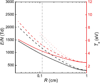
Figure 6. Reduced electric field (black curves; left axis) and electron temperature (red; right), as a function of the radius, calculated for p = 300 Pa,  cm−3 and
  K as follows: using the transport theory presented here, considering the influence of negative ions O− (solid curves); using the transport theory presented here, neglecting the influence of negative ions O− (dashed); adopting the classical ambipolar diffusion theory (dotted). The dashed–dotted vertical line limits the R-region of low pressure conditions.
Download figure:
Standard image High-resolution imageRecall that the description presented in section 2.1.1, of the ambipolar transport for a dense plasma with multiple positive ions, has assumed similar temperatures, drift velocities, and collision frequencies for all positive ions. This approximation has been checked using the results of simulations for the main positive ions O , NO+, O+ and N
 (X) (see section 4.2), by estimating the differences in the velocities of each species and by comparing their net creation frequencies, calculated as
Calculations show that (i) the differences in the velocities of the i-ion species, expected to scale as  , range between
  (for the most abundant ions) and
  (between O
 and O+ , exhibiting the highest difference in mass); (ii) for each working condition, the differences between the various
  are below
  .
.
4.2. Results at various electron densities
This paper focuses on the self-consistent model of air plasmas, produced using microwaves (f = 2.45 GHz) within fused-silica capillaries (R = 345 μm) at low pressure (p = 300 Pa). In addition to p, R and f, simulations require also information on Tg and ne as input data (see section 3), and in the present study the values of these quantities are taken also from the experiment [20]. Figure 7 presents (i) typical measured values of the gas temperature and the electron density, used as input data in the simulations; (ii) the self-consistent reduced electric field, as a function of the electron density, as obtained from the simulations. The values of E/N depicted in this figure correspond to calculations using the transport theory described in section 2.1, considering or neglecting the influence of negative ion O−. As observed, the presence of these ions leads to a decrease of ∼400 Td in the reduced electric field (for all ne values considered), thus to a reduction in the rates of electron-impact ionization mechanisms in a situation where the charged-particle diffusion losses are also smaller (see figure 2).

Figure 7. Experimental gas temperature (black curve; left axis) and calculated reduced electric field (red; right), as a function of the electron density. The self-consistent results for E/N are obtained for typical working conditions (p = 300 Pa, R = 345 μm and (ne, Tg) as in the black curve), considering (solid curve) or neglecting (dashed) the influence of negative ions O− in transport.
Download figure:
Standard image High-resolution imageThe high intensity of the maintenance reduced electric field, combined with moderate ionization degrees of ∼10−4, are responsible for a non-equilibrium distribution of the electron energy. Figures 8(a) and (b) shows the eedf and the N2(X, ) vdf, respectively, calculated for
  corresponding to the working conditions of figure 7. Note the enhancement of the eedf tail, as the reduced electric field increases, which suggests the importance of electron-impact mechanisms in controlling the plasma kinetics. Note further the non-equilibrium features of the plasma, confirmed by the departure of the eedfs from a Maxwellian distribution (check also the insert in figure 8(a), corresponding to a zoom over the low-energy region), and by the vdfs of N2(X).

Figure 8. (a) Electron energy distribution function and (b) vibrational distribution function of N2(X, ), calculated for the working conditions of figure 7, corresponding to the following E/N values in Td: 1560 (——), 1250 (- - - -), 630 (
 ). The dashed red-line in (a) is a Maxwellian distribution at Te = 5.7 eV, corresponding to the electron temperature of the eedf calculated at E/N = 1250 Td. The insert in (a) is a zoom over the low-energy region.
Download figure:
Standard image High-resolution imageFigures 9–12 present, as a function of the electron density and for the working conditions of figure 7, the calculated densities of the plasmas species associated with the following systems: molecular nitrogen and oxygen neutral species; atomic nitrogen and oxygen neutral species; nitrogen and oxygen ion species; and nitrogen oxide neutral species, respectively. Tables 3–7 present the most relevant kinetic mechanisms included in the model, corresponding to all reactions contributing more than  to the creation / destruction rates of each species, for all the working conditions considered here. The wall recombination / deactivation coefficients presented in these tables were adjusted to improve the agreement between model predictions and experimental diagnostics (see companion paper on the experimental investigation of these micro-plasmas [20]), but are within the predictable range for fused-silica [114], considering the higher wall-losses expected under the present low-pressure small-radius conditions.

Figure 9. Densities of molecular nitrogen and oxygen neutral species, as a function of the electron density, calculated for the same conditions as in figure 7. (a) Nitrogen species: N2(X) (black solid line), N2(A) (red solid), N2(B) (red dashed), N2(C) (red dotted), N2(a') (blue solid), N2(a) (blue dashed). N2(w) (blue dotted). (b) Oxygen species: O2(X) (black solid line), O2(a) (red solid), O2(b) (red dashed), O3 (blue solid), O (blue dashed).
Download figure:
Standard image High-resolution image
Figure 10. Densities of atomic neutral species, as a function of the electron density, calculated for the same conditions as in figure 7. Oxygen species: O(3P) (black solid line), O(1D) (black dashed); nitrogen species N(4S) (red solid), N(2D) (red dashed), N(2P) (red dotted).
Download figure:
Standard image High-resolution image
Figure 11. Densities of nitrogen and oxygen ions, as a function of the electron density, calculated for the same conditions as in figure 7. (a) Nitrogen ions: N (X) (black solid line), N
 (B) (black dashed), N+ (red solid), N
 (red dashed)
  (red dotted). (b) Oxygen and NO ions: O
 (black solid line), O+ (black dashed), O− (black dotted), NO+ (black dashed-dotted).
Download figure:
Standard image High-resolution image
Figure 12. Densities of nitrogen oxide neutral species, as a function of the electron density, calculated for the same conditions as in figure 7. NO(X) (black solid line), NO(A) (black dashed), NO(B) (black dotted), NO2(X) (red solid), NO2(A) (red dashed).
Download figure:
Standard image High-resolution image
Table 3. Summary of the most important creation / destruction reactions of molecular nitrogen.
| No. | Reaction | k (cm3s−1) | Reference |
|---|---|---|---|
| MN1 | e + N2(X) → e + N2(A,B,C,a,a',w) | f (E/N) | [53] |
| MN2 | e + N2(A) → e + N2(C) | f (E/N) | [64] |
| MN3 | N2(B) + N2 → N2(A) + N2 |  |
[35, 90] |
| MN4 | N2(a) + N2 → N2(a') + N2 |  |
[91] |
| MN5 | N2(w) + N2 → N2(a) + N2 | 10−11 | [92] |
| MN6 | N2(a) + O2 → N2(X) + 2O(3P) |  |
[91] |
| MN7 | N2(B) + O2 → N2(X) + 2O(3P) |  |
[74] |
| MN8 | N2(w) + O2 → N2(X) + 2O(3P) | 10−10 | [35] |
| MN9 | N2(A) + N2(X, ) → N2(B) + N2(X, ) → N2(B) + N2(X, ) ) |
 |
[35] |
| MN10 | N2(C) → N2(B) + hν |  |
[93] |
| MN11 | N2(B) → N2(A) + hν |  |
[94] |
| MN12 | N2(A, B, C, a, a', w) + wall → N2(X) |  |
|
aEmission frequency in s−1. bWall deactivation coefficient. Note: The label f (E /N) means that the rate coefficient is calculated by integration of the corresponding cross section over the eedf.
Table 4. Summary of the most important creation / destruction reactions of molecular oxygen.
| No. | Reaction | k (cm3s−1) |
Reference |
|---|---|---|---|
| MO1 | e + O2(X) → e + O2(a,b) | f (E/N) | [53] |
| MO2 | e + O2(a)  e + O2(b) e + O2(b) |
f (E/N) | [49, 69] |
| MO3 | e + O2(a) → e + O2(X) | f (E/N) | [53, 63] |
| MO4 | e + O2(a) → 2e + O |
f (E/N) | [53] (see section 2.2.1) |
| MO5 | e + O3 → e + O(3P) + O2(X) | f (E/N) | [49] (see section 2.2.1) |
| MO6 | e + O2(a,b) → e + O(3P) + O(3P) | f (E/N) | [53] (see section 2.2.1) |
| MO7 | O(1D) + O2(X) → O(3P) + O2(b) |  |
[39] |
| MO8 | O− + O2(X) → e + O3 | 10−12 | [82] |
| MO9 | O− + O2(a) → e + O3 |  |
[39, 83] |
| M10 | O− + O → e + O2 |  |
[82] |
| MO11 | O + 2O2 → O + O2 + O2 |
 |
[39, 95] |
| MO12 | O2(a) + O → 2O2(X) + O → 2O2(X) + O |
 |
[96] |
| MO13 | O + O → 2O2(X) → 2O2(X) |
 |
[95] |
| MO14 | O2(b) + wall → O2 |  |
|
| MO15 |  + wall → O3 + wall → O3 |
 |
|
aFor three-body reactions, the rate coefficient is in cm6 s−1. bWall deactivation coefficient. Note: In this table, Tg is in K. The label f (E /N) has the same meaning as in table 3.
Table 5. Summary of the most important creation / destruction reactions of atomic nitrogen and oxygen.
| No. | Reaction | k (cm3s−1) | Reference |
|---|---|---|---|
| A1 | e + N2(X) → e + N(4S) + N(4S,2D) | f (E/N) | [65] |
| A2 | e + O2(X) → e + O(3P) + O(3P,1D) | f (E/N) | [53] |
| A3 | e + N(4S) → e + N(2D,2P) | f (E/N) | [61] |
| A4 | e + N(2D) → e + N(2P) | f (E/N) | [67] |
| A5 | e + O(3P) → e + O(1D) | f (E/N) | [62] |
| A6 | N(2P) + N2(X,v  ) → N(4S) + N2(A) ) → N(4S) + N2(A) |
 |
[73] |
| A7 | O(3P), N(4S) + wall → 1/2O2, 1/2N2 |  |
|
| A8 | N(2D, 2P) + wall → N(4S) |  |
|
| A9 | O(1D) + wall → O(3P) |  |
|
aWall recombination coefficient. bWall deactivation coefficient. Note: In this table, Tg is in K. The label f(E/N) has the same meaning as in table 3.
Table 6. Summary of the most important creation / destruction reactions of nitrogen, oxygen and nitrogen oxide ions.
| No. | Reaction | Obs. |
|---|---|---|
| I1 | e + N2(X) → 2e + N (X,B) (X,B) |
R1 in tables A1 and A4 |
| I2 | e + N(4S,2D) → 2e + N+ | R23 in table A1 |
| I3 | e + O2(X,a) → 2e + O |
R1, R2 in table A2 |
| I4 | e + O(3P) → 2e + O+ | R7 in table A2 |
| I5 | e + O2(X) → 2e + O+ + O(3P) | R8 in table A2 |
| I6 | e + NO(X) → 2e + NO+ | R16 in table A2 |
| I7 | N + N2(A) → N + N2(A) → N + N + N |
R10 in table A1 |
| I8 | N + N2(X,v = 0) + N2(X) → + N2(X,v = 0) + N2(X) →  + N2 + N2 |
R11 in table A1 |
| I9 | N2(A,a') + N2(a') → e +  |
R16, R17 in table A1 |
| I10 | N+ + N2(X,v = 0) + N2(X) → N + N2 + N2 |
R31 in table A1 |
| I11 | N (B) → N (B) → N (X) + hν (X) + hν |
R3 in table A4 |
| I12 | e + O2(X,a) → O− + O | R1, R2 in table A3 |
| I13 | O− + O → O2 + e | R6 in table A3 |
| I14 | O− + N2(X) → N2 + O(3P) + e | R7 in table A3 |
| I15 | O− + O2(X) → O3 + e | R3 in table A3 |
| I16 | e + O− → O(3P) + 2e | R12 in table A3 |
| I17 | O− + O+ → O + O | R14 in table A3 |
| I18 |  + O2(X) → O + O2(X) → O + N2 + N2 + N2 + N2 |
R19 in table A1 |
| I19 | N+ + O2 → O + N + N |
R25 in table A1 |
| I20 | N+ + O2 → NO+ + O | R26 in table A1 |
| I21 | N+ , N , N , N , ,  + wall → N, N2, N2 + N, 2N2 + wall → N, N2, N2 + N, 2N2 |
R37-R40 in table A1 |
| I22 | O+ , O , NO+ + wall → O, O2, NO , NO+ + wall → O, O2, NO |
R18-R20 in table A2 |
Table 7. Summary of the most important creation / destruction reactions of nitrogen oxide species.
| No. | Reaction | k (cm3s−1) |
Reference |
|---|---|---|---|
| NO1 | NO+ + wall → NO(X) | ||
| NO2 | N2(X, 13) + O(3P) → N(4S) + NO(X) 13) + O(3P) → N(4S) + NO(X) |
10−13 | [97] |
| NO3 | e + NO(X) → 2e + NO+ | f (E/N) | [58] |
| NO4 | NO(X) + N(4S) → N2(X, ) + O(3P) ) + O(3P) |
 |
[97] |
| NO5 | NO(X) + N2(a') → N2(X) + N + O |  |
[74] |
| NO6 | NO(X) + N(2D) → N2(X) + O(3P) |  |
[98] |
| NO7 | NO(X) + O → NO+ + O2 → NO+ + O2 |
 |
[74] |
| NO8 | NO(X) + N2(A) → N2(X,v = 0) + NO(A) |  |
[99] |
| NO9 | NO(A) → NO(X) + hν |  |
[100, 101] |
| NO10 | NO(A) + N2 → NO(X) + N2 | 10−13 | [102–105] |
| NO11 | N(4S) + O(3P) + O2 → NO(B) + O2 |  |
[106] |
| NO12 | N(4S) + O(3P) + N2 → NO(B) + N2 |  |
[106] |
| NO13 | NO(B) NO(X) + hν NO(X) + hν |
 |
[106] |
| NO14 | NO(B) + N2 → NO(X) + N2 |  |
[103, 105, 107] |
| NO15 | NO(B) + O2 → NO(X) + O2 |  |
[103, 105, 107, 108] |
| NO16 | NO(B) + NO → NO(X) + NO |  |
[103, 105, 108, 109] |
| NO17 | NO(X) + O− → NO2(X) + e |  |
[82] |
| NO18 | NO2(X) + O(3P) → NO(X) + O2 |  |
[110] |
| NO19 | O(3P) + NO(X) + O2 → NO2(A) + O2 |  |
[111, 112] |
| NO20 | O(3P) + NO(X) + N2 → NO2(A) + N2 |  |
[111, 112] |
| NO21 | NO2(A) + O2 → NO2(X) + O2 |  |
[112] |
| NO22 | NO2(A) + N2 → NO2(X) + N2 |  |
[113] |
aFor three-body reactions, the rate coefficient is in cm6 s−1. bEmission frequency in s−1. Note: In this table, Tg is in K. The label f (E/N) has the same meaning as in table 3.
The results in figures 9(a) and (b) reveal that N2(X) and O2(X) are the most abundant species, as expected. Note that, depending on the electron density, molecular nitrogen exhibits densities 4.5–6 times higher than those of molecular oxygen, the initial air-mixture composition containing only 4 times more N2 than O2, as a consequence of the larger dissociation degree for oxygen. Figures 9(a) and (b) shows also that O2(a), O2(b) and N2(A), N2(B) are the dominant excited species, with densities ∼ 1014 cm−3 and ∼ 1012 cm−3, respectively, and that O3 has a very low density, 5-6 orders of magnitude below that of O2(X), as expected keeping in mind the high gas temperatures and the low-pressure discharge conditions under investigation. The kinetics of the dominant molecular neutral species is controlled (i) in nitrogen, mainly by electron-impact excitation from N2(X) and by diffusion and wall deactivation (check reactions MN1 and MN12 in table 3), and in the case of N2(B,C) also by radiative transitions (MN10 and MN11); (ii) in oxygen, mainly by electron-impact excitation, ionization and dissociation (check reactions MO1–MO6 in table 4), and in the case of O2(b) also by quenching O(1D) with O2(X) (MO7) and by diffusion and wall deactivation (MO14).
At low E/N (hence low ne) electron-impact mechanisms become less effective, which explains the increase of N2(X) and O2(X) as the electron density decreases. The higher concentrations of these molecules at low electron density enhance the losses of the N2 excited states via quenching with N2 and dissociative quenching with O2 (MN3–MN9). However, although the densities of N2(B, C, a, w) decrease as ne decreases, the concentrations of N2(A) and N2(a') are maintained through reactions MN3 and MN4, which become important source channels for these species at low electron density (see figure 9(a)). In oxygen at low ne, the quenching of excited states with O2 ground-state species is less important. Indeed, the excitation transfer MO7 between oxygen atoms and molecules becomes the most important mechanism as the electron density decreases, being responsible for the slight increase in the populations of both O2(b) and O2(a) (also via MO2) (see figure 9(b)).
Figure 9(a) reveals an inversion in the populations of the N2(A) and N2(B) states, as the electron density increases. The phenomenon is caused by the highly-active electron kinetics under the present working conditions, for which  eV (see figure 6). In fact, numerical tests confirm that it is possible to avoid the population inversion by setting to zero the rate coefficients of the direct electron-impact excitation of N2(A,B,C), yet keeping their creation via heavy-species collisions. The result can be further explained by analyzing the theoretical prediction for the density ratio of these states, in a situation exclusively controlled by electron-impact elastic, inelastic and superelastic collisions, in which case their populations would follow a Boltzmann distribution at temperature Te

where  and
and  are the statistical weights of states N2(A) and N2(B), respectively, and
  eV and
  eV are the corresponding excitation energies. Equation (27) shows that an inversion in the populations of these states is expected for
  eV, i.e. well below the typical ∼ 6 eV characterizing the temperature of electrons in the present situation. Obviously, the complete kinetic modeling of N2-O2 low-pressure plasmas in capillaries is influenced by more than just electron-impact mechanisms. As seen, heavy-particle reactions (strongly dependent on the gas temperature, not the electron temperature) and the transport of species both play a fundamental role in the results. For example, the non-equilibrium features induced by these mechanisms contribute to a difference by a factor of about 10−4 between the populations of N2(X) ground-state and N2(A,B) excited states (see figure 9(a)), well below the ratio [N2(A,B)] / [N2(X)] ≃1–2 (corresponding to a population inversion also with respect to the ground-state), obtained under an equilibrium situation at
  eV. Actually, the influence of the heavy-particle dynamics is observed also at low electron density (see figure 9(a)), where electron scattering can no longer induce a N2(A)–N2(B) population inversion.
Figure 10 shows that O(3P) is the most abundant atomic species, with a density of ∼ 1015 cm−3, followed by N(4S) and O(1D) with densities ∼20 times lower. These results confirm the high dissociation degree of oxygen ([O(3P)]/[O2(X)] ∼20%–70%, for  cm−3), in contrast with the [N(4S)]/[N2(X)] ∼0.1% dissociation reported for nitrogen. The main creation channels of the dominant atomic species are electron-impact dissociation and excitation (check reactions A1–A5 in table 5), which explains the increase in their densities with ne. The main destruction mechanism for these species is by diffusion and wall recombination / deactivation (A7–A9), and for the excited state N(2P) is also by quenching with higher-lying vibrational levels of N2 (A6).
Figures 11(a) and (b) shows that O , NO+ and O+ (the latter at high ne) are the most abundant ion species, followed by N
 (X) and the negative ion O− whose populations are already ∼10 times below the electron density. As expected, the main creation channel for the dominant positive ions is by electron-impact ionization (check reactions I1–I6 in table 6), whereas the main destruction mechanism is by diffusion and wall recombination (I21–I22). The radiative emission (I11) plays an important role in the creation / destruction of N
 (X) and N
 (B). Similarly to the atomic species, the densities of O
 , O+ , N
 (X,B), N+ and N
 increase with ne, due to the ruling of electron-impact mechanisms in the creation of these species. However, the densities of positive ions NO+ and
  behave differently when the electron density increases: (i) NO+ is created mainly by electron-impact ionization I6, but its density remains almost constant due to the decrease in the concentration of the parent neutral species NO(X) with ne (see figure 12); (ii)
  is created mainly via the three-body reaction I8 involving the ground-state N2(X), whose density decreases with ne (see figure 9).
The main creation / destruction mechanisms of the negative ion O− are dissociative attachment (I12) and associative detachment (I13), respectively. At low electron density, the higher concentrations of N2(X) and O2(X) make the losses of O− to depend also of reactions I14 and I15, but the stronger attachment rate associated with I12 is ultimately responsible for an increase in the density of the negative ion.
The most abundant species with the NO system is NO(X), with a density (2– cm−3, followed by NO2(X) with a density 300–500 times lower, as can be observed in figure 12. The main creation / destruction mechanisms of these species are: for NO(X), wall recombination and electron-impact ionization (check reactions NO1 and NO3 in table 7); for NO2(X), associative detachment and dissociation by impact with O-atoms (NO17 and NO18). Note that collisions of ground-state oxygen atoms with N2(A) and of ground-state oxygen molecules with N(2D) contribute less than
  to the formation of NO(X), contrary to what is observed for example in microwave plasmas produced in centimeter-radius tubes at pressures of 102–103 Pa [113]. In general, the kinetics of the nitrogen oxide system is controlled by collisions between heavy species, namely: (i) ground-state atoms O(3P), N(4S) and molecules N2(X), playing an important role in the creation of NO(B) and NO2(A) (NO12 and NO20) and in the destruction of NO2(X) and NO2(A) (NO18 and NO22); (ii) the nitrogen excited state N2(A), responsible for the excitation of NO(A) from NO(X) (NO8). The radiative decays NO9 and NO13 are the main destruction channels of NO(A) and NO(B), respectively. As outcome, the populations of the nitrogen oxide species are affected only indirectly by the electron density, exhibiting small variations with changes in ne.
5. Final remarks
This work presented the self-consistent modeling of microwave (f = 2.45 GHz excitation frequency) micro-plasmas, produced in dry air ( ) within capillaries (R = 345 μm inner radius) at low gas pressure (p = 300 Pa). The study used the LoKI numerical code, an in-house simulation tool that couples the homogeneous two-term EBE with the 0D rate balance equations for the most relevant charged and neutral species of the plasma. The code uses as input data the experimental values of the electron density (
 –
– cm−3) and the gas temperature (
 –1000 K) [20], in addition to f, R and p, calculating the self-consistent reduced electric field E/N by imposing the quasi-neutrality condition, and adjusting the relative composition of the mixture after the dissociation of molecular species, while ensuring a constant pressure value. Note that a full self-consistent description of the plasma should include a thermal model, to calculate the gas temperature as part of the numerical solution, which is scheduled as a next step of this research program. A very complete thermal model should also consider different ion temperatures, as the outcome of the ion recombination and the energy deposition on the small-radius discharge tube, with impact on the formulation of the charged-particle transport model.
The transport of charged particles, under the extreme conditions of small-radius low-pressure adopted here, was described using the bases of the unified transport theory for dense plasmas at various pressures proposed by Self and Ewald [28], and later reinterpreted by Ferreira and Ricard [29]. This theory, originally set for plasmas containing a single positive ion species, was revised here so as to consider the presence of several positive ions and a negative ion with low density. In particular, (i) the transport of the total positive charge in the plasma was described using a single effective positive ion; (ii) the model formulation was limited to low/intermediate pressures, considering vanishingly small attachment/detachment rates, in which case the low-density negative ion has negligible drift velocity and remains confined to the plasma core. Under these hypothesis, we have retrieved a system of equations formally identical to that of [28], whose solution can be worked-out from the original results of Self and Ewald, yielding a correction upon the abacus  versus
  obtained in [29]. For the typical low-pressure working conditions considered here, this correction is sufficient to modify the relative characteristic diffusion length, the reduced maintenance electric field and the electron temperature of the air micro-plasmas under study, even at electron to negative-ion density ratios as small as 0.05. At larger discharge radii, the self-consistent population of O− becomes negligible, and the current transport formulation can still be used to give the asymptotic values predicted by the classical ambipolar diffusion theory for
  ,
,  , E/N and Te.
The description of the plasma chemistry required the study of the stable quaternary mixture N2:O2:N:O, namely when solving the EBE. We have revised the very complete kinetic schemes presented in [47, 48] for nitrogen and in [35, 49] for oxygen and for N2–O2 mixtures, particularly the mechanisms of charged-particle creation / destruction that have special relevance for maintaining the highly-excited plasma. In this context, the electron-impact scattering cross sections from ground-state molecular / atomic nitrogen and oxygen were also revised and extended to 1 keV. These sets of cross sections are or will become shortly available on the IST-LISBON database of LXCat [52]. The model considers also other electron scattering cross sections, for mechanisms not conserving the number of electrons and/or for inelastic/superelastic collisions (including dissociation) with excited states, namely N2(A,B,C), N(4S,2D,P) and O2(a,b), which can play an important role in defining the plasma chemistry.
Model results at various ne show that the most abundant neutral species are N2(X) and O2(X) (with densities of ∼(2– cm−3 and ∼(2–
 cm−3, respectively); O(3P) (∼(1–
 cm−3); NO(X) (∼(2–
 cm−3); O2(a), O2(b) and O(1D), N(4S) (∼1014 cm−3 and ∼
 cm−3, respectively); and N2(A), N2(B) (∼1012 cm−3). These results confirm the high dissociation degree of oxygen ([O(3P)]/[O2(X)] ∼20%–70%, in contrast with only [N(4S)]/[N2(X)] ∼0.1% dissociation for nitrogen. Moreover, the model predicts a very low density for O3, which is found 5–6 orders of magnitude below that of O2(X), as expected considering the present high-temperature low-pressure conditions. The kinetics of the dominant neutral species with nitrogen and oxygen is controlled mainly by electron-impact reactions (excitation, ionization, dissociation), by radiative transitions and by diffusion and wall deactivation / recombination. At low electron densities, the quenching of excited species by N2(X) and O2(X) becomes a competitive mechanism. The main creation / destruction mechanisms of NO(X) are wall recombination of NO+ and electron impact ionization, respectively. The most abundant ion species are O
 and NO+ (with densities of ∼1012 cm−3); O+ (∼1011–1012 cm−3, as ne varies between
  cm−3); and N
 (X) and O− (∼1011 cm−3). The positive ion species are created mainly by electron-impact ionization and are destroyed mainly by diffusion and wall recombination, the FNS radiative emission playing also an important role in the creation of N
 (X) from N
 (B). The main creation / destruction mechanisms of the negative ion O− are dissociative attachment and associative detachment, respectively.
The modeling of air micro-plasmas presented here can contribute to deepen the knowledge on these systems, particularly in what concerns the identification of the most important species controlling the plasma maintenance. The extreme small-radius low-pressure conditions adopted have allowed to study pure (rare-gas-free)  plasmas, and have also put forward specific creation / destruction paths dominated by electron-impact collisions and by diffusion and wall deactivation / recombination, respectively. Accordingly, the LoKI numerical code was successfully adapted to describe the transport of charged-particles in ambipolar weakly electronegative plasmas, adopting a strategy easy to be implemented in other studies dealing with similar working conditions. The code is to be validated, by comparing simulation results with experimental diagnostics of the line-emission intensities and the absolute densities of several relevant molecular and atomic plasma species. The conclusions of this validation procedure will be presented in the second part of this work, to be published in a follow-up paper.
Acknowledgments
This work was partially supported by Portuguese FCT—Fundação para a Ciência e a Tecnologia, under Project UID/FIS/50010/2013, and by Project PLASMA-ADIST. L L Alves benefited from an FCT scholarship (SFRH/BSAB/1360/2013) to carry out this work. The authors thank G Stancu, O Leroy, K Gadonna and T Minea for providing the experimental data used as input parameters in the simulations.
Appendix.: Tables with kinetic schemes for the ions
Table A1. Kinetic scheme for ground-state nitrogen ions N+ , N , N
, N and
and  .
.
| No. | Reaction | k (cm3s−1)a | Reference |
|---|---|---|---|
| R1 | e + N2(X) → 2e + N |
f (E/N) | [53] |
| R2 | e + N2(A) → 2e + N |
f (E/N) | [66] |
| R3 | e + N2(a') → 2e + N |
f (E/N) | [64] |
| R4 | e + N2(B) → 2e + N |
f (E/N) | [64] |
| R5 | e + N2(a) → 2e + N |
f (E/N) | [64] |
| R6 | e + N2(w) → 2e + N |
f (E/N) | [64] |
| R7 | N(2D) + N(2P) → e + N |
10−13 | [73] |
| R8 | e + N (X) → N(4S) + N(4S) (X) → N(4S) + N(4S) |
 |
[74] |
| R9 | N + N(4S) + N2 → N + N(4S) + N2 → N + N2 + N2 |
 |
[74] |
| R10 | N + N2(A) → N + N2(A) → N + N + N |
 |
[74] |
| R11 | N + N2(X,v = 0) + N2 → + N2(X,v = 0) + N2 →  + N2 + N2 |
 |
[75] |
| R12 | N + O2(X) → O + O2(X) → O + N2(X,v = 0) + N2(X,v = 0) |
 |
[74] |
| R13 | N + O(3P) → NO+ + N(4S) + O(3P) → NO+ + N(4S) |
 |
[74] |
| R14 | N + O(3P) → O+ + N2(X,v = 0) + O(3P) → O+ + N2(X,v = 0) |
 |
[74] |
| R15 | N + NO(X) → NO+ + N2(X,v = 0) + NO(X) → NO+ + N2(X,v = 0) |
 |
[74] |
| R16 | N2(A) + N2(a') → e +  |
10−11 | [76] |
| R17 | N2(a') + N2(a') → e +  |
 |
[76] |
| R18 | e +  → N2(v = 0) + N2(v = 0) → N2(v = 0) + N2(v = 0) |
 |
[74] |
| R19 |  + O2(X) → O + O2(X) → O + N2 + N2 + N2 + N2 |
 |
[74] |
| R20 |  + O(3P) → O+ + N2 + N2 + O(3P) → O+ + N2 + N2 |
 |
[74] |
| R21 |  + NO → NO+ + N2 + N2 + NO → NO+ + N2 + N2 |
 |
[74] |
| R22 |  + N2 → N + N2 → N + N2(X,v = 0) + N2 + N2(X,v = 0) + N2 |
 |
[77] |
| R23 | e + N(4S,2D,2P) → 2e + N+ | f (E/N) | [61] |
| R24 | O+ + N(2D) → N+ + O |  |
[74] |
| R25 | N+ + O2 → O + N + N |
 |
[74] |
| R26 | N+ + O2 → NO+ + O |  |
[74] |
| R27 | N+ + NO → N + NO+ |  |
[74] |
| R28 | N+ + N2(X,v 4) → N(4S) + N 4) → N(4S) + N |
 |
[78] |
| R29 | N+ + O + N2 → NO+ + N2 | 10−29 | [74] |
| R30 | N+ + O + O2 → NO+ + O2 | 10−29 | [74] |
| R31 | N+ + N2(X,v = 0) + N2 → N + N2 + N2 |
 |
[79] |
| R32 | N2(a') + N(2P) → N + e + e |
10−11 | [80] |
| R33 | N + O2 → O + O2 → O + N + N2 + N + N2 |
 |
[74] |
| R34 | N + N(4S) → N + N(4S) → N + N2 + N2 |
 |
[74] |
| R35 | N + NO → NO+ + N + N2 + NO → NO+ + N + N2 |
 |
[74] |
| R36 | N + e → N2 + N + e → N2 + N |
 |
[74] |
| R37 | N+ + wall → N | ||
| R38 | N + wall → N2(X) + wall → N2(X) |
||
| R39 | N + wall → N2(X) + N(4S) + wall → N2(X) + N(4S) |
||
| R40 |  + wall → 2N2(X) + wall → 2N2(X) |
aFor three-body reactions, the rate coefficient is in cm6s−1. Note: In this table, Tg and Te are in K. The label f (E/N) means that the rate coefficient is calculated by integration of the corresponding cross section over the eedf.
Table A2. Kinetic scheme for oxygen-containing positive ionsa O+ , O and NO+.
| No. | Reaction | k (cm3s−1)b | Reference |
|---|---|---|---|
| R1 | e + O2(X) → 2e + O |
f (E/N) | [53] |
| R2 | e + O2(a) → 2e + O |
f (E/N) | [53] (see section 2.2.1) |
| R3 | e + O → O(3P) + O(3P) → O(3P) + O(3P) |
 |
[74] |
| R4 | e + O → O(3P) + O(1D) → O(3P) + O(1D) |
 |
[39] |
| R5 | O + N(4S) → NO+ + O(3P) + N(4S) → NO+ + O(3P) |
 |
[74] |
| R6 | O + NO(X) → NO+ + O2(X) + NO(X) → NO+ + O2(X) |
 |
[74] |
| R7 | e + O(3P) → 2e + O+ | f (E/N) | [62] |
| R8 | e + O2(X) → 2e + O+ + O(3P) | f (E/N) | [70] |
| R9 | e + O2(a) → 2e + O+ + O(3P) | f (E/N) | [70] (see section 2.2.1) |
| R10 | O+ + NO(X) → NO+ + O(3P) |  |
[81] |
| R11 | O+ + N2(X,v = 0) + O2(X) → NO+ + N(4S) + O2 |  |
[74] |
| R12 | O+ + N2(X,v = 0) + N2(X) → NO+ + N(4S) + N2 |  |
[74] |
| R13 | O+ + O2(X) → O + O(3P) + O(3P) |
 |
[77] |
| R14 | O+ + O2(a) → O + O(3P) + O(3P) |
 |
[39, 50] |
| R15 | O+ + O3 → O + O2(X) + O2(X) |
10−10 | [74] |
| R16 | e + NO(X) → 2e + NO+ | f (E/N) | [58] |
| R17 | e + NO+ → N + O |  |
[77] |
| R18 | O+ + wall → O | ||
| R19 | O + wall → O2 + wall → O2 |
||
| R20 | NO+ + wall → NO |
aThis kinetic scheme is to be completed with reactions from tables A1, A3 and A4. bFor three-body reactions, the rate coefficient is in cm6s−1. Note: In this table, Tg and Te are in K. The label f (E/N) has the same meaning as in table A1.
Table A3. Kinetic scheme for oxygen negative ion O−.
| No. | Reaction | k (cm3s−1)a | Reference |
|---|---|---|---|
| R1 | e + O2(X) → O− + O | f (E/N) | [53] |
| R2 | e + O2(a) → O− + O | f (E/N) | [71] |
| R3 | O− + O2(X) → O3 + e | 10−12 | [82] |
| R4 | O− + O2(a) → O3 + e |  |
[39, 83] |
| R5 | O− + O2(b) → O + O2 + e |  |
[39] |
| R6 | O− + O → O2 + e |  |
[82] |
| R7 | O− + N2(X) → N2O + e | 10−11 | [82] (see section 2.2.2) |
| R8 | O− + N2(A) → O + N2 + e |  |
[39] |
| R9 | O− + N2(B) → O + N2 + e |  |
[39] |
| R10 | O− + N(4S) → NO + e |  |
[82] |
| R11 | O− + NO → NO2 + e |  |
[82] |
| R12 | e + O− → O(3P) + 2e | f (E/N) | [72] |
| R13 | O− + O → O2 + O → O2 + O |
 |
[39] |
| R14 | O− + O+ → O + O |  |
[84] |
| R15 | O− + N+ → N + O |  |
[74] |
| R16 | O− + N+ + N2 → O + N + N2 |  |
[74] |
| R17 | O− + N+ + N2 → NO + N2 |  |
[74] |
| R18 | O− + N+ + O2 → O + N + O2 |  |
[74] |
| R19 | O− + N+ + O2 → NO + O2 |  |
[74] |
| R20 | O− + N → N + N2 + O → N + N2 + O |
10−7 | [74] |
aFor three-body reactions, the rate coefficient is in cm6 s−1. Note: In this table, Tg is in K and the label f(E/N) has the same meaning as in table A1.
Table A4. Kinetic scheme for nitrogen excited ion N (B).
(B).
| No. | Reaction | k (cm3s−1) | Reference |
|---|---|---|---|
| R1 | e + N2(X,v = 0) → 2e + N (B,v = 0) (B,v = 0) |
f (E/N) | [68] |
| R2 | e + N (X,v = 0) → e + N (X,v = 0) → e + N (B,v = 0) (B,v = 0) |
f (E/N) | [68] |
| R3 | N (B) → N (B) → N (X) + hν (X) + hν |
 a a |
[85] |
| R4 | N2(X,v ) + N ) + N (X) → N (X) → N (B) + N2(X,v-12) (B) + N2(X,v-12) |
10−11 | [77, 86] |
| R5 | N (B) + wall → N2 (B) + wall → N2 |
aEmission frequency in s−1. Note: In this table, the label f (E/N) has the same meaning as in table A1.