


ABSTRACT
The magnetic and velocity field fluctuations in magnetohydrodynamic turbulence can be characterized by their directional alignment and induced electric field. These manifest as coherent spatial correlations which are measures of Alfvénicity and turbulence cascade strength, respectively. Solar wind observations and direct numerical simulations find that these distinctive correlations, caused by rapid relaxation processes that act to suppress nonlinearity, occur in localized spatial patches. This cellularization of magnetofluid turbulence is inconsistent with a superposition of Gaussian fields and could be related to spatial intermittency or other non-Gaussian statistics.
Export citation and abstract BibTeX RIS
1. INTRODUCTION
A distinctive feature of fluid-scale plasma fluctuations as observed by spacecraft in the solar wind is the presence of so-called Alfvénic correlation (Belcher & Davis 1971; Bruno et al. 1985; Roberts et al. 1987). This is the familiar correlation of magnetic and velocity field fluctuations that is reminiscent of propagating small amplitude waves (Barnes 1979). It is also a property of large-amplitude propagating solutions to the incompressible magnetohydrodynamic (MHD) equations when superposed on a uniform background magnetic field (Parker 1979). The Alfvénic correlation observed in the solar wind inside of 1 AU usually has the same orientation associated with outward traveling waves. Hence, these correlations have been interpreted as waves that originated near the Sun and are convected outward in the supersonic solar wind (Belcher & Davis 1971; Velli & Grappin 1991). These "Alfvén waves" are fundamental in linear theory. However, it has been known for some time that the same correlation appears as a preferred global state in nonlinearly evolving MHD plasma (Dobrowolny et al. 1980; Matthaeus & Montgomery 1980; Pouquet et al. 1986). This dynamic alignment of magnetic and velocity field fluctuations leads to a type of global turbulence relaxation that is often encountered but not universal (Ting et al. 1986; Stribling & Matthaeus 1991). Such global dynamic alignment is not found in solar wind observations, which instead show that interplanetary plasma evolves with increasing distance from the Sun toward a less Alfvénic state on average. This is possibly due to driving by large-scale shear flows (Roberts et al. 1991).
Numerical simulations have shown (Matthaeus et al. 2008; Servidio et al. 2008) that Alfvénic correlations can occur in random patches and with random sense of alignment. If the appearance of such patches is a fundamental property of magnetofluid turbulence, then evidence for them might be found in the solar wind. This present study examines the appearance of random localized Alfvénic patches in both simulations and solar wind data obtained near Earth orbit at 1 AU. We find that MHD simulations, sampled along a linear trajectory to mimic single spacecraft measurements, and solar wind observations show patches that exhibit highly variable characteristics. Therefore, the presence of these localized spatial patches means that the local magnetic and velocity field correlation need not coincide with the global estimate, neither in magnitude nor degree of alignment. In particular, a global alignment with a large averaged cross helicity does not necessarily mean that simple interpretations in terms of Alfvén waves are valid.
The rest of the paper is structured as follows. Section 2 describes the solar wind data selection criteria and details of the MHD simulation. It also presents the analysis techniques used to obtain the results in Section 3. We will focus primarily on probability distributions showing the alignment and anti-alignment of magnetic and velocity field fluctuations, which derive from entire data sets and from selected subsamples. Direct comparisons will be made between the solar wind and numerical simulation results. A summary and discussion of these results is presented in Section 4.
2. DATA SELECTION AND ANALYSIS
We are concerned here with the properties of the magnetic and velocity field fluctuations,  and
and  , where
  and
and  are the total velocity and magnetic field vectors, respectively, and the angle brackets 〈...〉 designate an ensemble averaging operator that is typically substituted by a suitable time average. The main diagnostics used in this study of directional alignment are probability density functions (PDFs) of the local sine and cosine of the angle θ between
  and
and  , that is,

Note that cos θ is a measure of Alfvénic correlations (Belcher & Davis 1971) and sin θ can be interpreted as a measure of the induced electric field which drives the MHD turbulence cascade associated with the induction equation (Marsch & Tu 1992). We choose an arbitrary reference direction associated with unit vector  , conveniently taken in the solar wind case to be in the radial direction. It is assumed that a right-handed Cartesian system is employed in evaluating
  , sum implied over indices i, j, and l.
While the PDFs of cos θ and sin θ usefully highlight different characteristics of solar wind turbulence, they are not independent. Indeed, these distributions are related analytically such that if one is known, the other can be determined. Therefore, since the sin θ PDFs do not contain any new information, it is instructive to also compute the induced electric field directly:

This arises from the fluctuating magnetic and velocity fields, and is important when considering the structure and dynamics of MHD turbulence.
2.1. Solar Wind
We analyze the entire 64 s resolution magnetic and velocity field data sets from the Magnetic Field Experiment (MAG; Smith et al. 1998) and Solar Wind Electron, Proton, and Alpha Monitor (SWEPAM) (McComas et al. 1998) instruments on board the Advanced Composition Explorer (ACE) spacecraft. A natural ensemble is obtained by dividing the data into 10 hr intervals. This duration is long enough to contain several correlation times, but short enough to avoid large-scale inhomogeneities. In order to maintain statistical stationarity, intervals are removed from the ensemble if they contain heliospheric current sheet crossings or transient events such as shocks. Intervals are also discarded if the amount of missing or bad data exceeds 5%, since this would reduce the statistical robustness of any computed quantities. The remaining intervals number 156 and contain around 85,000 data points and constitute our solar wind data set for the present study. Each of the data intervals is sector rectified such that positive values of normalized cross helicity and cos θ correspond to outward (anti-sunward) "propagating" Alfvénic fluctuations. This convention is also extended to the sign associated with values of sin θ.
2.2. MHD Simulation
We also carried out numerical simulation of incompressible three-dimensional (3D) MHD turbulence for which the following equations were solved:

where  is the velocity field,
  is the fluctuating magnetic field, and p* is the total (fluid + magnetic) pressure determined by the incompressibility condition. The kinematic viscosity and magnetic diffusivity are ν and η, respectively. The simulation has unit magnetic Prandtl number (i.e., ν = η).
The fluctuations evolve in the presence of a uniform and static external magnetic field that is taken to be in the z-direction, i.e.,  . The non-dimensionality is such that, for the chosen initial conditions, B20 is the ratio of the energy density associated with
  to that associated with the initial magnetic fluctuations (
 at t = 0).
The magnetic helicity,  , where
  , in the simulation run is approximately zero at all times. However, the run is initially set up with some finite cross helicity,
  . A convenient dimensionless measure is the normalized cross helicity, σc ≡ 2Hc/E, where the energy
  . Here, the angle brackets indicate spatial averaging.
Initial conditions for the simulation run are generated in Fourier space. The amplitudes of  are chosen so that the modal kinetic energy is described by
where C is a normalization constant. In order to determine the phase of each  , the real and imaginary parts are assigned using independent Gaussian random variables. Usually only a subset of the retained Fourier modes is populated initially, that is, only those lying between limiting values, e.g., kL ⩽ k ⩽ kH. Initial conditions for
  are chosen in a similar way. However, controlling the degree of correlation between
  and
and  allows the cross helicity to be specified. The total energy E in the simulation is initially unity and is equipartitioned between Ev and Eb at all scales.
In Table 1 the parameters for the simulation run are summarized.
Table 1. Parameters Representing the MHD Simulation
| Grid | ν, η | B0 |  |
σc(t = 0) | σc(t = 2) |
|---|---|---|---|---|---|
| 5123 | 0.001 | 1.0 | 1.6 | 0.23 | 0.30 |
Notes. The initially excited Fourier modes have wavenumbers k ∈ [1, 5] and use k0 = 3 in the spectral shape function. kmax is the maximum retained dynamical wavenumber and kdiss is the dissipation wavenumber (reciprocal of the Kolmogorov scale).
Download table as: ASCIITypeset image
3. RESULTS
3.1. Global Statistics
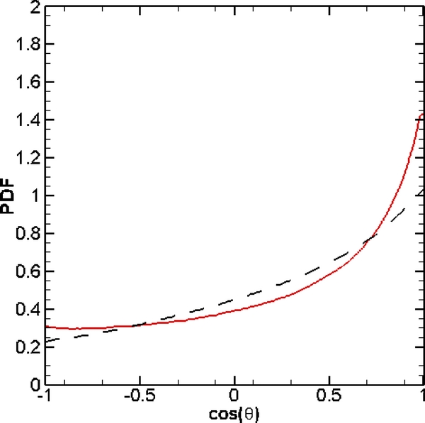
The 156 intervals that compose our entire solar wind data set are combined in order to analyze their global ensemble characteristics. A normalized cross helicity of 0.29 is obtained, which suggests a dominance of outward propagating fluctuations. This is consistent with expectations and suggests that our data set contains a representative sample of the ecliptic solar wind at 1 AU. Figure 1 shows (solid line) the PDF of cos θ which corresponds to the global behavior of solar wind turbulence. It shows probability enhancements associated with the alignment and anti-alignment of magnetic and velocity field fluctuations. While there is a preference for outward propagating Alfvénic fluctuations, there is a weak minority component of inward propagating fluctuations. This asymmetry is a consequence of the non-zero net cross helicity of solar wind turbulence at 1 AU. For comparison, Figure 1 also shows the PDF (dashed line) of cos θ from the entire spatial domain of the 3D MHD simulation. The normalized cross helicity associated with the simulation is around 0.3, which is comparable to the solar wind case. Indeed, both PDFs behave in a similar manner and are characterized by strong enhancements associated with the alignment of magnetic and velocity field fluctuations. Hence, the PDFs in Figure 1 are consistent with local dynamic alignment and MHD turbulence relaxation toward global evolution of Alfvénic states (Dobrowolny et al. 1980; Pouquet et al. 1986; Ting et al. 1986; Stribling & Matthaeus 1991; Matthaeus et al. 2008; Servidio et al. 2008).

Figure 1. PDFs of cos θ from the entire solar wind data set (solid line) and MHD simulation spatial domain (dashed line). The associated normalized cross helicities are σc = 0.29 and σc = 0.30, respectively, indicating a preponderance of outwardly "propagating" Alfvénic fluctuations in the solar wind case. The general form of both PDFs is similar, showing significant probability enhancements associated with alignment of magnetic and velocity field fluctuations. Note that the PDF of cos θ is flat when θ is the angle between two vectors with random orientations.
Download figure:
Standard image High-resolution imageFigure 2 shows PDFs of sin θ from the solar wind data set (solid line) and MHD simulation (dashed line), further characterizing the global behavior of magnetofluid turbulence. In both cases, the PDFs show significant probability increases linked to induced electric field fluctuations, which are perpendicular to both the magnetic and velocity field fluctuations.

Figure 2. PDFs of sin θ from the entire solar wind data set (solid line) and MHD simulation spatial domain (dashed line). The probability enhancements shown are indicative of a strong induced electric field, and the behavior of both PDFs is nearly identical. Note that pdf(sin θ) = pdf(cos θ) · |tan θ|.
Download figure:
Standard image High-resolution imageThe global properties of the induced electric field are also examined directly. For the solar wind data set, the induced electric field vector is determined in Radial Tangential Normal (RTN) coordinates. Figure 3(a) shows the PDF of the radial component. The exponential character of the electric field distribution is consistent with previous studies (Breech et al. 2003; Sorriso-Valvo et al. 2004). The induced electric field vector is also computed from the MHD simulation, and Figure 3(b) shows the PDF of the z component ez. Since the Reynolds number in the solar wind is orders of magnitude greater than that achieved in the MHD simulation, events with large induced electric field values are more likely. Induced electric field strength can be used as a measure of the strength of turbulent couplings in a magnetofluid such as the solar wind. A simple estimate is its standard deviation, equal to the root-mean-square (rms) fluctuation:

A heuristic measure of the fluctuating electric field strength can be made by normalizing δe by the rms magnetic and velocity field fluctuations, respectively, δb and δv. Using the entire solar wind data set, δe is about 95% of the product δvδb. This implies a strong induced electric field. Since the electric field helps drive the MHD turbulence cascade, our results indicate the presence of active turbulence dynamics in the solar wind despite the appearance of Alfvénic correlations. Note that the presence of an active cascade in the solar wind has been confirmed by computation of third-order statistics (see Smith et al. 2009; Marino et al. 2011, and references therein), employing the extension of the Kolmogorov–Yaglom law to MHD (Politano & Pouquet 1998).
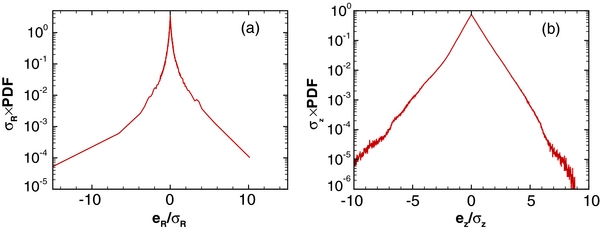
Figure 3. Normalized PDF of the induced electric field (a) radial component from the entire solar wind data set, where σR is the standard deviation of eR, and (b) z-component from the 3D MHD simulation, where σz is the standard deviation of ez.
Download figure:
Standard image High-resolution image3.2. Local Statistics
Here we examine the cross helicity content derived from smaller samples of solar wind and simulation data. In order to facilitate ease of comparison across these data sets, it is desirable that the 3D simulation emulate the one-dimensional (1D) spacecraft data. Therefore, the magnetic and velocity fields are sampled along a linear trajectory through the MHD simulation domain (Greco et al. 2008). The computation is simplified by aligning the trajectories along a Cartesian axis. Each 1D path through the simulation extends to about 12 correlation lengths (integral scales). This is chosen to match the 10 hr intervals of solar wind data which, assuming an average speed of 400 km s−1 and a correlation length of 1.2 × 10⁶, correspond to around the same spatial scale.
Each 10 hr interval within our solar wind data set is analyzed for evidence of local directional alignment. The left-hand column of Figure 4 shows PDFs of cos θ for three intervals which correspond to localized spatial patches of solar wind turbulence. These particular intervals were selected to illustrate the breadth of σc variability within our data set. The solar wind interval associated with the top panel has a normalized cross helicity of 0.75, and consists almost solely of outward-directed Alfvénic alignments and partial alignments. This is reflected in the PDF which has a substantial probability increase linked to alignment of the magnetic and velocity field fluctuations, but has no population of anti-aligned fluctuations. Despite the presence of these strong Alfvénic correlations, the induced electric field associated with this data interval represents about 54% of δvδb, indicating a significant and active turbulence cascade. The middle panel represents a solar wind interval with a normalized cross helicity of 0.17, which contains a mixture of both inward and outward fluctuations. Consequently, the PDF shows probability enhancements associated with both alignment and anti-alignment of magnetic and velocity field fluctuations. An induced electric field is also present and constitutes about 65% of the product δvδb, which suggests the turbulence dynamics are strong. In contrast to the top panel, the bottom panel is linked to a solar wind interval with a normalized cross helicity of −0.73, which consists almost entirely of inward-directed Alfvénic correlations. The PDF has a significant probability increase connected to the anti-alignment of the magnetic and velocity fluctuations, but has no population of aligned fluctuations. However, the presence of an induced electric field within this data interval, which constitutes 49% of the product δvδb, implies a strongly driven turbulence cascade.
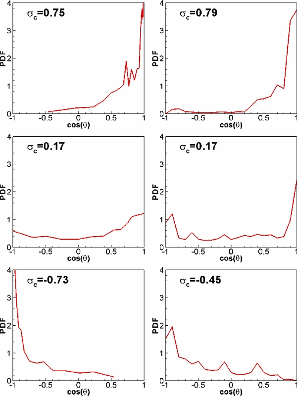
Figure 4. PDFs of cos θ from (left column) 10 hr intervals of solar wind data, and (right column) linear trajectory samples of 3D MHD simulation data. These PDFs correspond to localized spatial patches where the Alfvénic correlations have a dominant anti-sunward alignment (top), mixture of sunward–anti-sunward alignments (middle), and dominant sunward alignment (bottom).
Download figure:
Standard image High-resolution imageThe right-hand column of Figure 4 shows PDFs of cos θ for a selection of linear trajectory samples through the 3D MHD simulation. In order to compare with the results in the left-hand column, the simulation data that best matched the corresponding solar wind σc values were chosen. Figure 4 illustrates the good agreement between the simulation data PDFs and their solar wind counterparts. These cos θ distributions are consistent with directional alignment, the emergence of local Alfvénic states as a consequence of rapid turbulence relaxation.
While the PDFs shown in Figure 4 are computed from particular data intervals, they are typical of the variability in both the solar wind and MHD simulation data set. These results are consistent with the idea that MHD turbulence in general, and solar wind turbulence in particular, display a strong tendency to form localized spatial patches of directionally aligned Alfvénic fluctuations (Matthaeus et al. 2008). However, it is interesting to note that a strong induced electric field is maintained (as in Figure 3) despite the local evolution toward Alfvénic correlations. The strength of this electric field does weaken slightly with increasing cross helicity, although it remains significant. Since the electric field contributes to driving the MHD turbulence cascade, the appearance of partial Alfvénic states does not indicate a lack of turbulence dynamics. This is a feature that would not be expected when using a linear wave theory description. Therefore, drawing conclusions regarding the presence or importance of wave activity on the basis of  –
– correlation is problematic.
3.3. Phase Coherency
Phase randomization is a technique used in the study of turbulence (Servidio et al. 2008). Here it is used in order to demonstrate that the observed spatial patches of Alfvénic alignment are associated with phase coherency. Fourier coefficients of the dynamical variables  and
and  are used to form new functions
  and
and  that have the same power spectrum as the originals but with random phases. In addition, we require that
  and
and  have the same total cross helicity as
  and
and  . The result is that the new fields
  and
and  lack coherency, a property that originates from the nonlinear nature of MHD and is encoded in the phases of the expansion of Fourier coefficients. Hence, this procedure is expected to destroy the coherent spatial patches of locally large positive and negative cross helicities, which correspond to significant alignment and anti-alignment of magnetic and velocity field fluctuations.
Figure 5 shows PDFs of cos θ from the phase-randomized fields (dashed line) and the original fields (solid line). The PDFs of both have a bias toward alignment of magnetic and velocity field fluctuations, which is consistent with their equal values of positive cross helicity. However, the PDF corresponding to the original fields has a greater probability associated with highly aligned and anti-aligned fluctuations. Figure 5 illustrates the non-Gaussian nature of the observed cellularization of MHD turbulence since our results are inconsistent with a superposition of Gaussian fields. Indeed, the requirement of phase coherency implies that there could be a link between local relaxation processes and turbulence intermittency.
Figure 5. PDFs of cos θ from the 3D MHD simulation data (solid line) and phase-randomized data (dashed line).
Download figure:
Standard image High-resolution image
4. CONCLUSIONS AND DISCUSSIONS
We have examined the issue of directional alignment between the magnetic and velocity field fluctuations in MHD turbulence using solar wind observations and direct numerical simulations. The solar wind data set used in this study was obtained at 1 AU and selected to be free of transient events and significant data gaps. The simulation initial data are such that they produce a global cross helicity that is similar to that of the solar wind data set. When the simulation reaches a strongly turbulent state, after being advanced in time, the resulting probability distributions of cos θ broadly match those obtained from the observational data. Indeed, the similarity in Alfvénic alignment distributions is among many features of the solar wind fluctuations that seem congruent with a turbulence description (Tu & Marsch 1995; Bruno & Carbone 2005; Matthaeus & Velli 2011).
When linear trajectory samples comprising a few correlation scales are extracted from the MHD simulation, the resulting distribution of cross helicity values is broad, extending almost over the full range of allowed values. This cross helicity content, along with the PDFs of cos θ for these simulation samples, indicates substantial variability. It is interesting that these properties of the MHD simulation are also reflected in the cross helicity values and cos θ distributions of the individual 10 hr intervals of solar wind data.
A consistent interpretation of these results is that the emergence of apparently Alfvénic local correlations are determined by the turbulence cascade, for both the solar wind and MHD simulation data, while the global correlation in both cases is determined by initial or boundary data. This understanding is based on recent studies (Matthaeus et al. 2008; Servidio et al. 2008) which found that rapid relaxation processes in MHD turbulence act to suppress nonlinearity by producing distinctive correlations that occur in localized spatial patches. We have shown that this cellularization of MHD turbulence is inconsistent with a superposition of jointly normal (Gaussian) fields. Hence, it could be related to spatial intermittency or other non-Gaussian statistics. This interpretation, which is supported by our results and previous studies, suggests that rapid relaxation and the emergence of non-Gaussian statistics are likely a dynamical property of solar wind fluctuations—a property shared with strong MHD turbulence.
This research is supported in part by the NSF Solar Terrestrial Program under grant AGS-1063439 and the NSF SHINE Program ATM-0752135, and by NASA under the Heliophysics Theory Program grant NNX08AI47G.